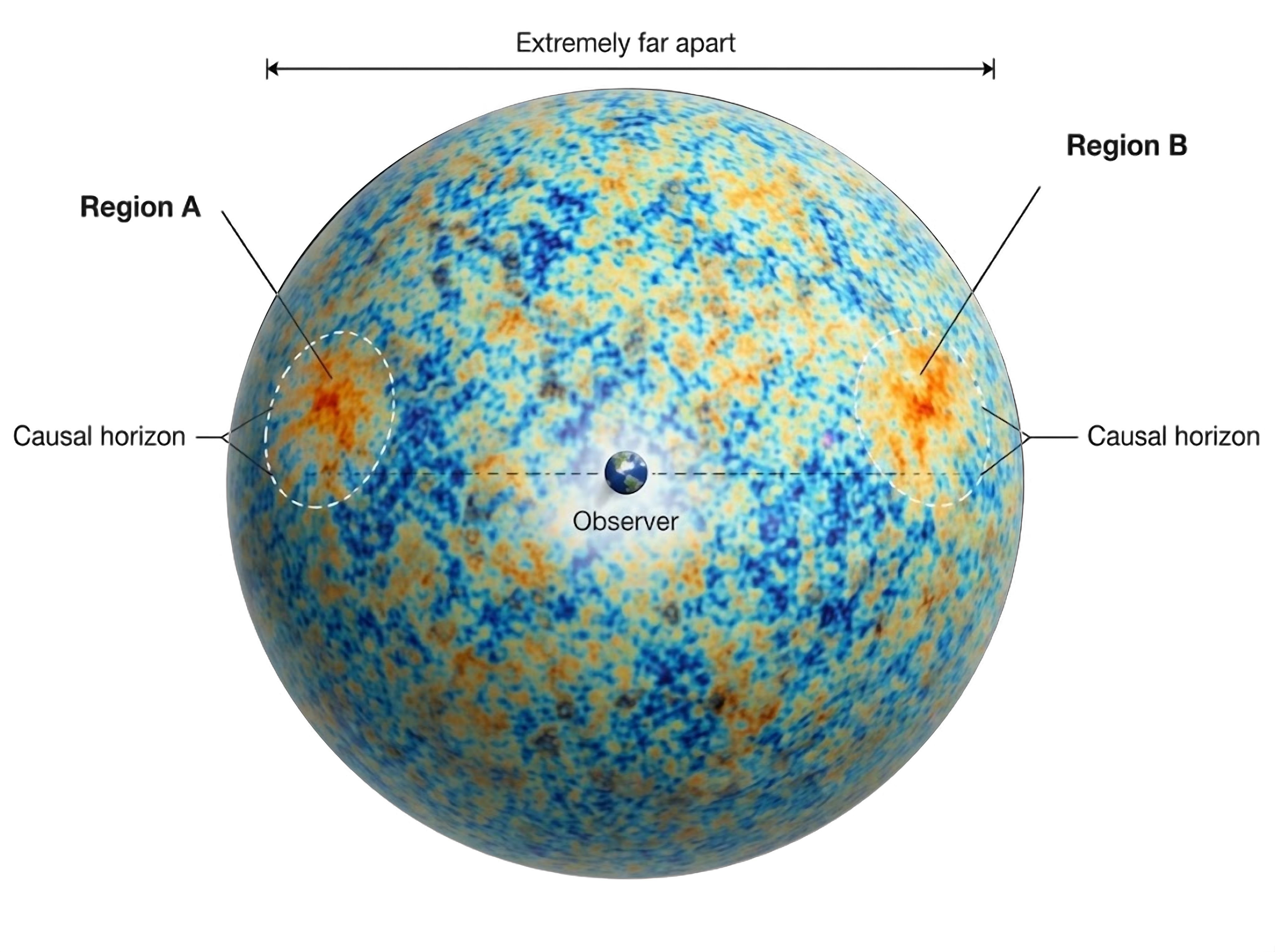
horizon
PhD defense, Université Paris Cité, 12 October 2026
Cosmic Microwave Background, Weak Lensing, and GPU-Accelerated Inference




Wassim KabalanUniversité Paris Cité, APC/CNRS
supervised by Eric Aubourg and Josquin Errard, co-advised by François Lanusse and Alexandre Boucaud
slides at askabalan.github.io/slides/2026_10_PhD
Stage 2 · SDSS, 2.5 m ground, 1.4″ seeing
Stage 4 · Euclid, 1.2 m space, 0.18″
Abell 2390 · Credit: SDSS DR18 (left); ESA / Euclid / Euclid Consortium / NASA, J.-C. Cuillandre & G. Anselmi (right)
Microwave
λ ≈ 1–10 mm

wavelength
Optical / near-infrared
λ ≈ 0.3–2 µm
Space based
Ground based
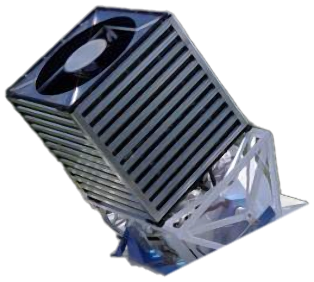
LiteBIRD
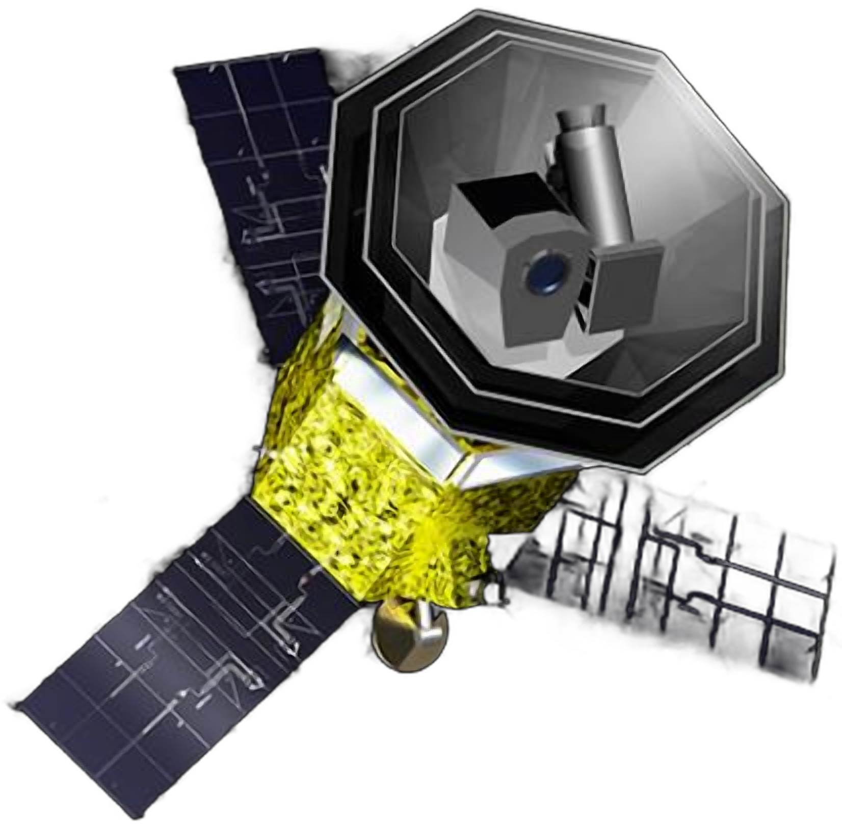
full sky, from space
12 bands, 40–402 GHz
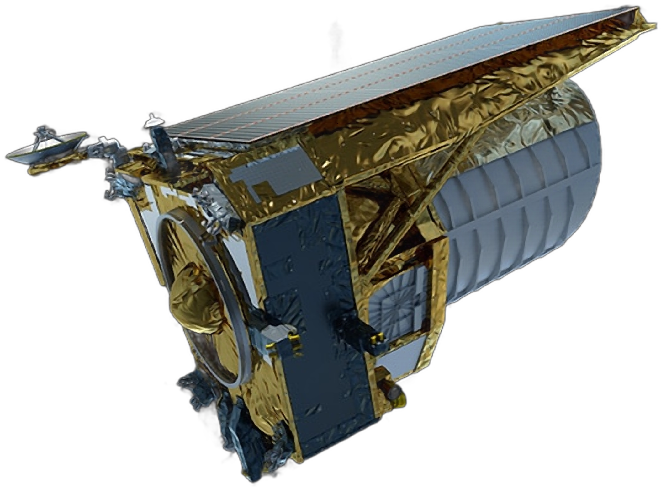
Euclid
14 000 deg²
30 gal arcmin⁻²
From Space
~1.5 billion galaxies
Simons Observatory
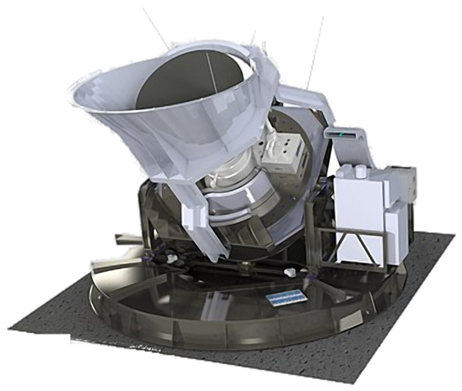
Atacama, Chile
6 bands, 27–280 GHz
Vera C. Rubin Observatory (LSST)
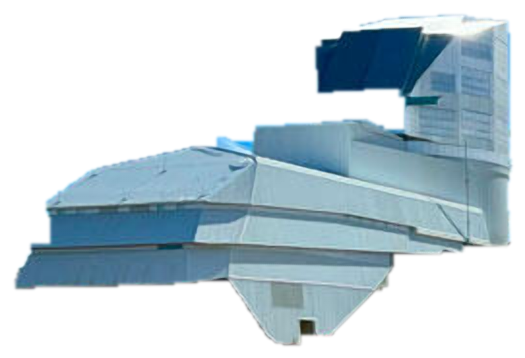
18 000 deg²
30 gal arcmin⁻²
Cerro Pachón in Chile
~2 billion galaxies




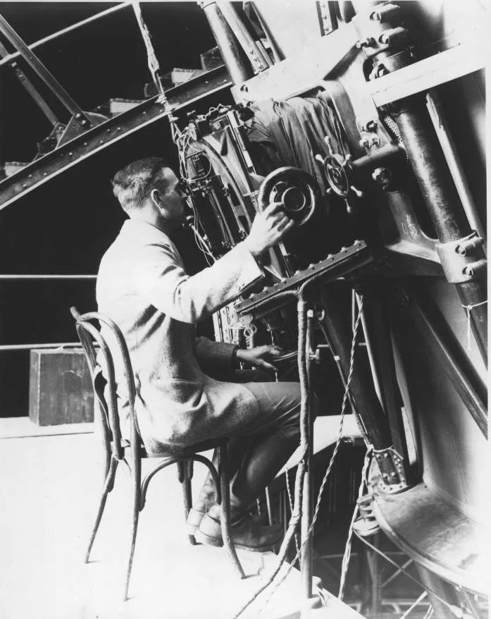
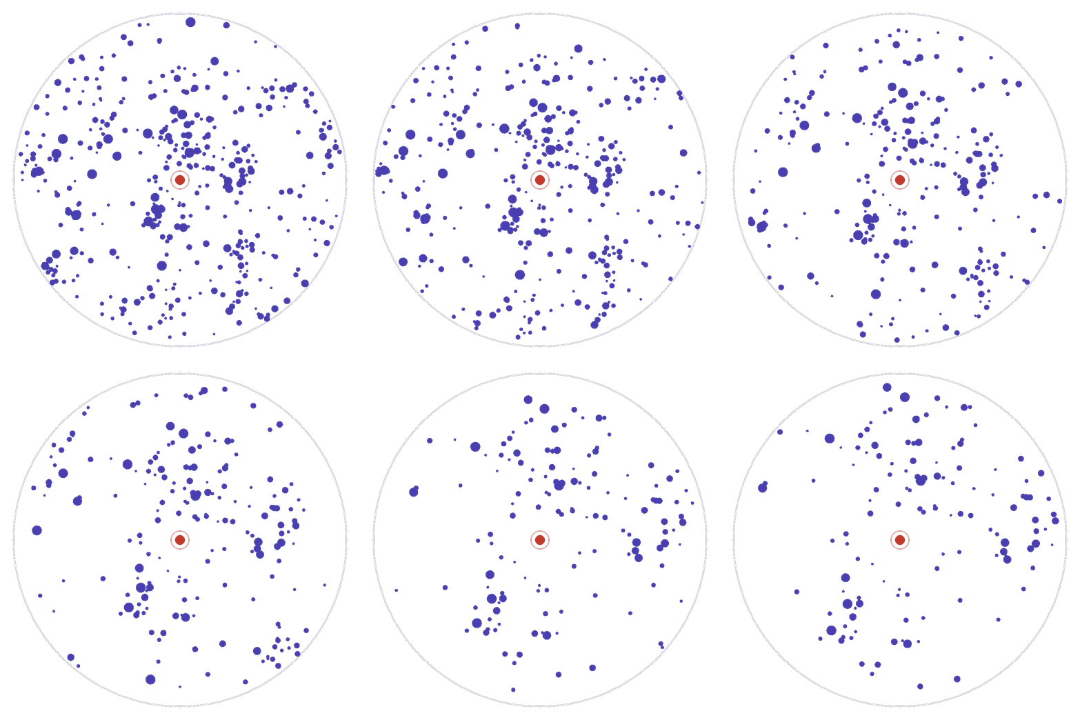
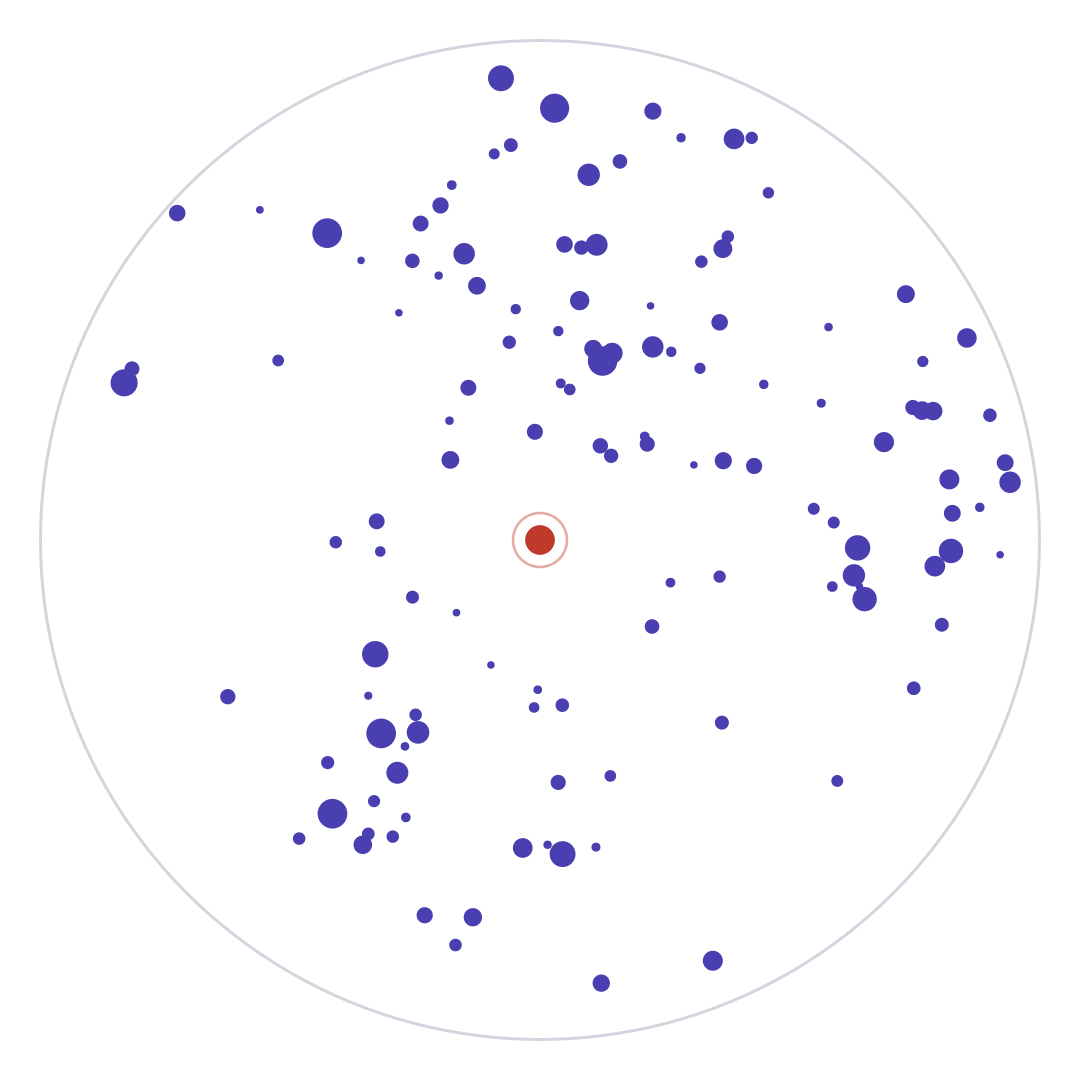
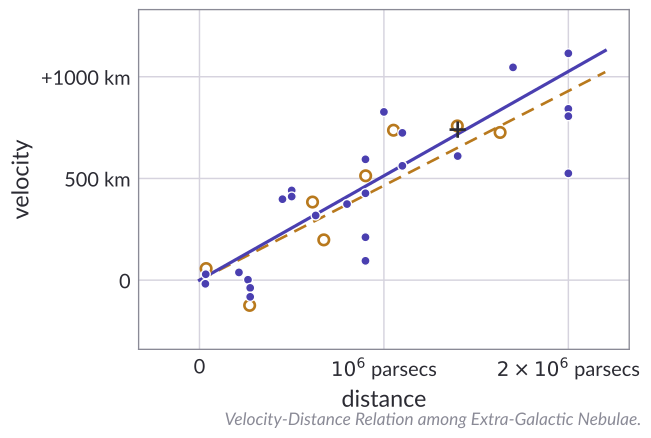
Credit: NASA (photograph); Hubble (1929), PNAS 15, 168, Fig. 1, redrawn
The Expanding Universe
Georges Lemaître: the Universe had a beginning
It expanded from an extremely dense early state
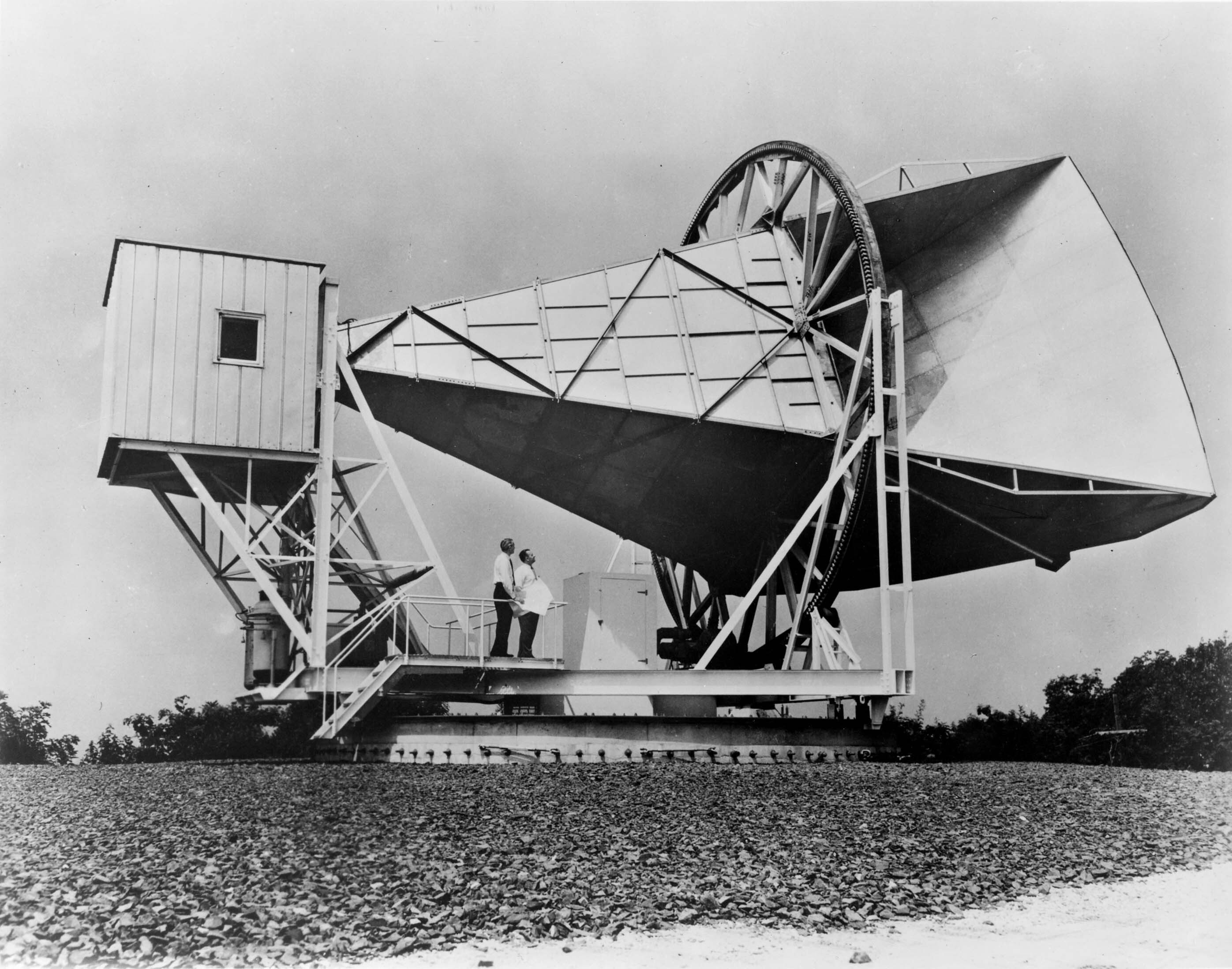
1965, Holmdel: Penzias & Wilson find a 3 K signal from every direction · Credit: NASA (antenna); ESA / Planck Collaboration (map)
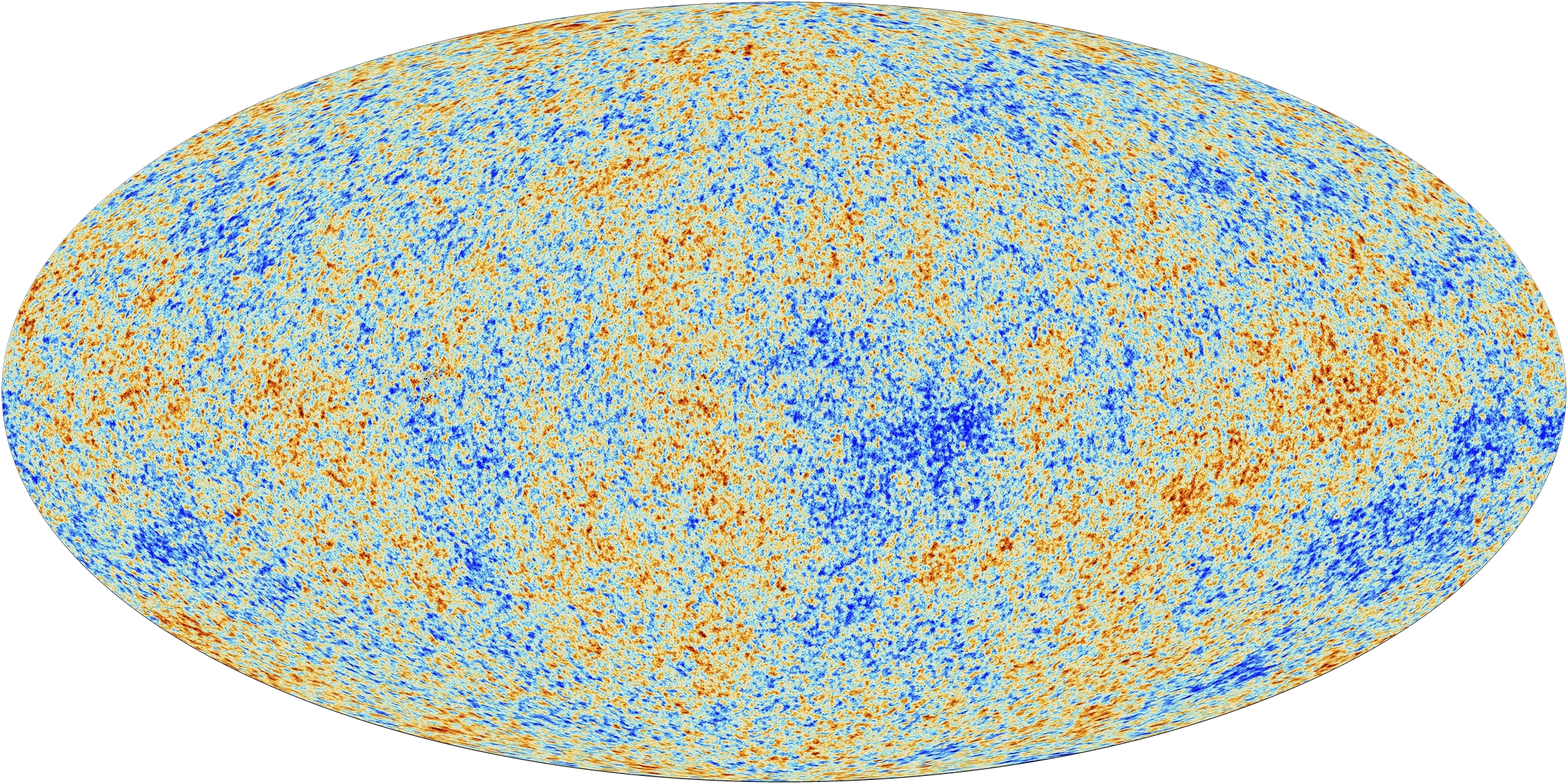
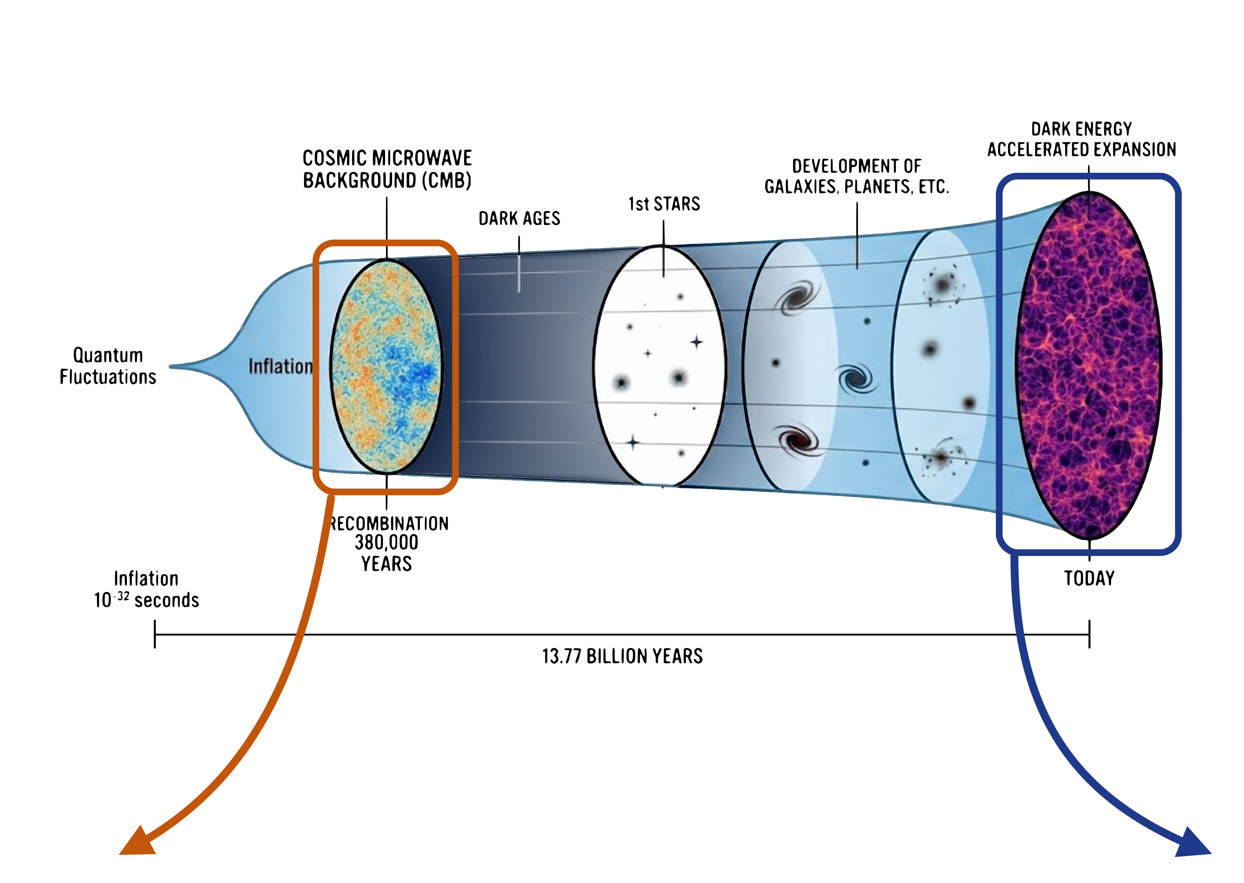
The CMB is one of the essential discoveries that confirm the hot Big Bang
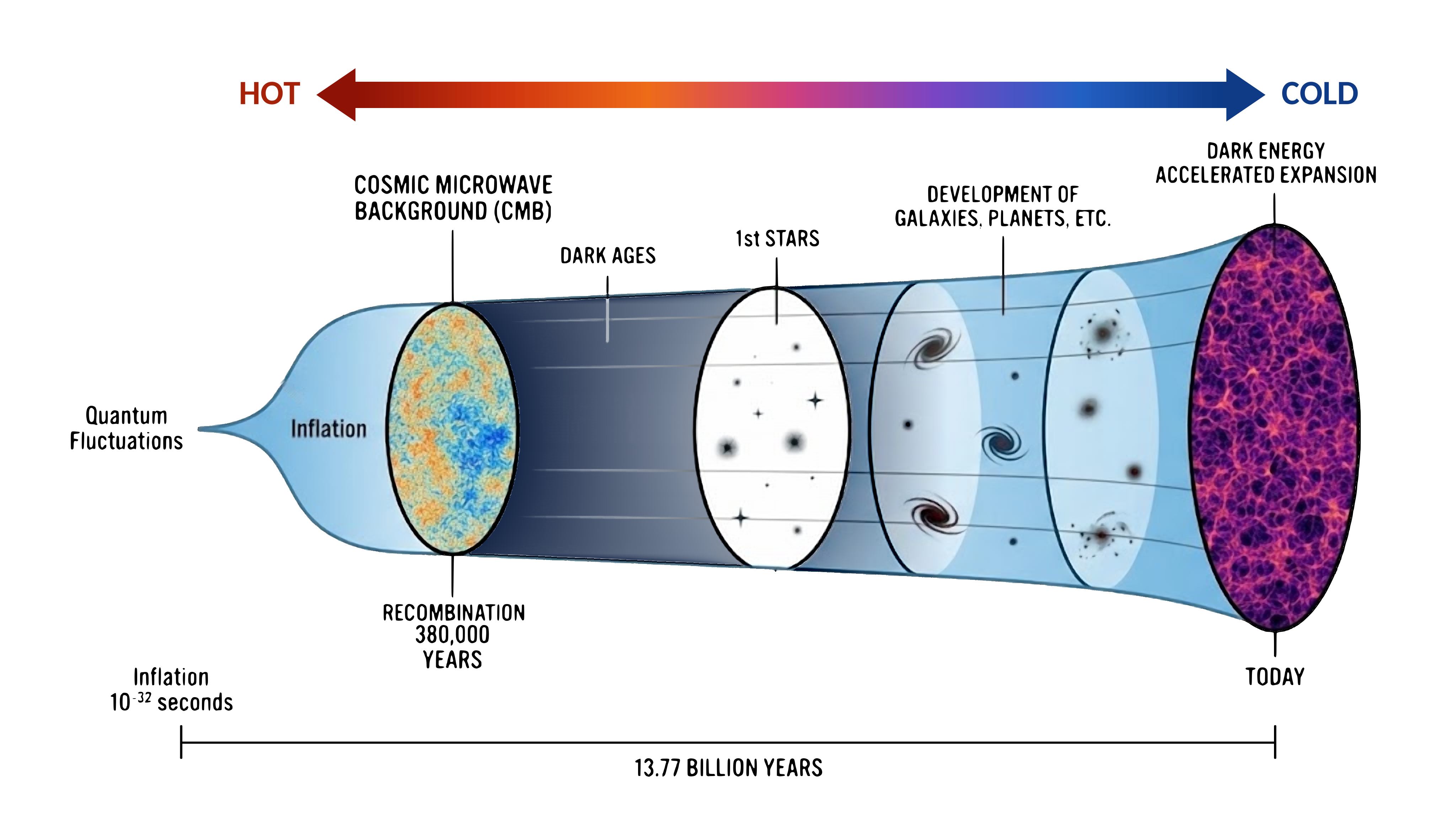

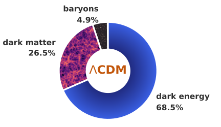
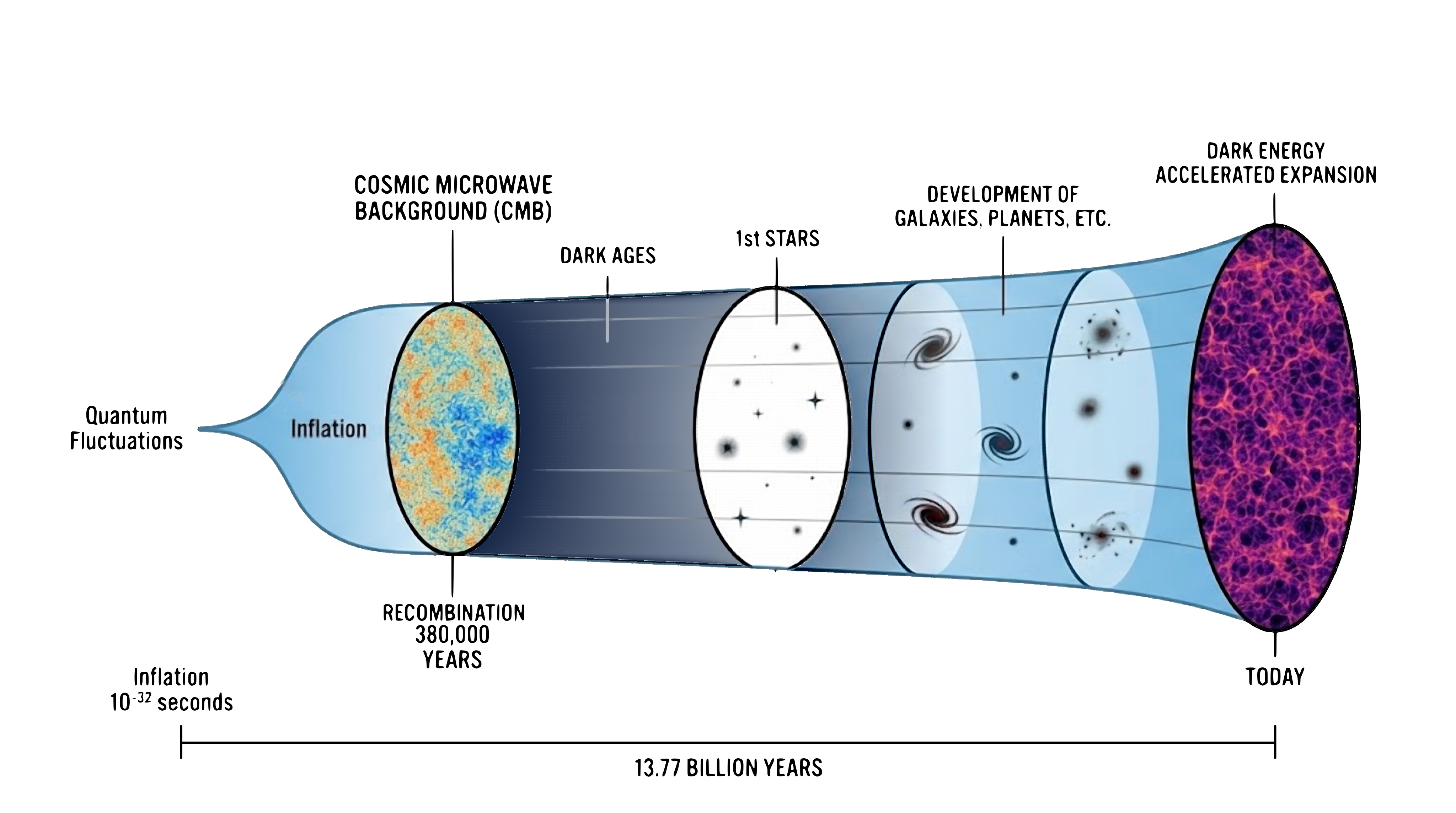
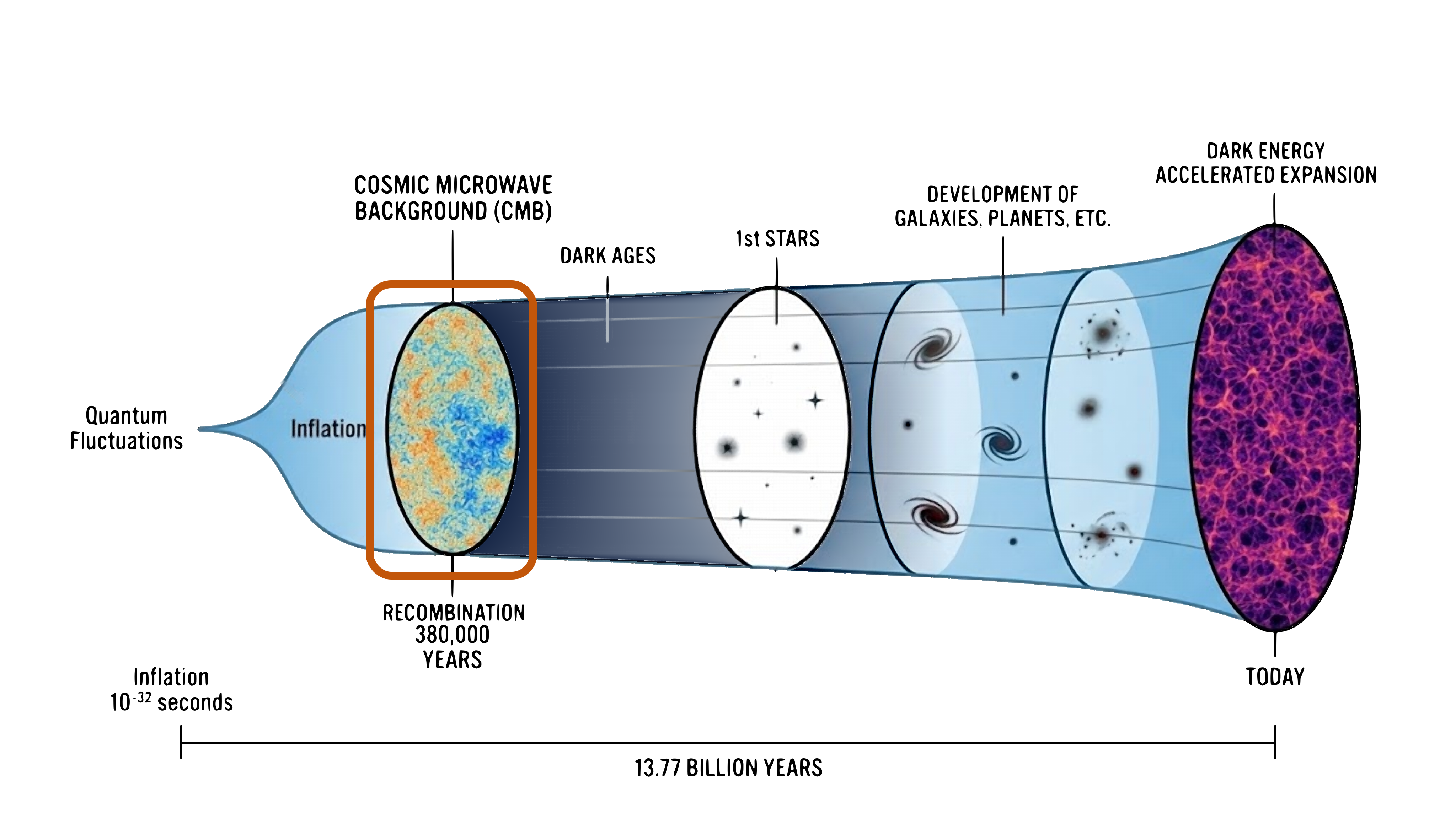
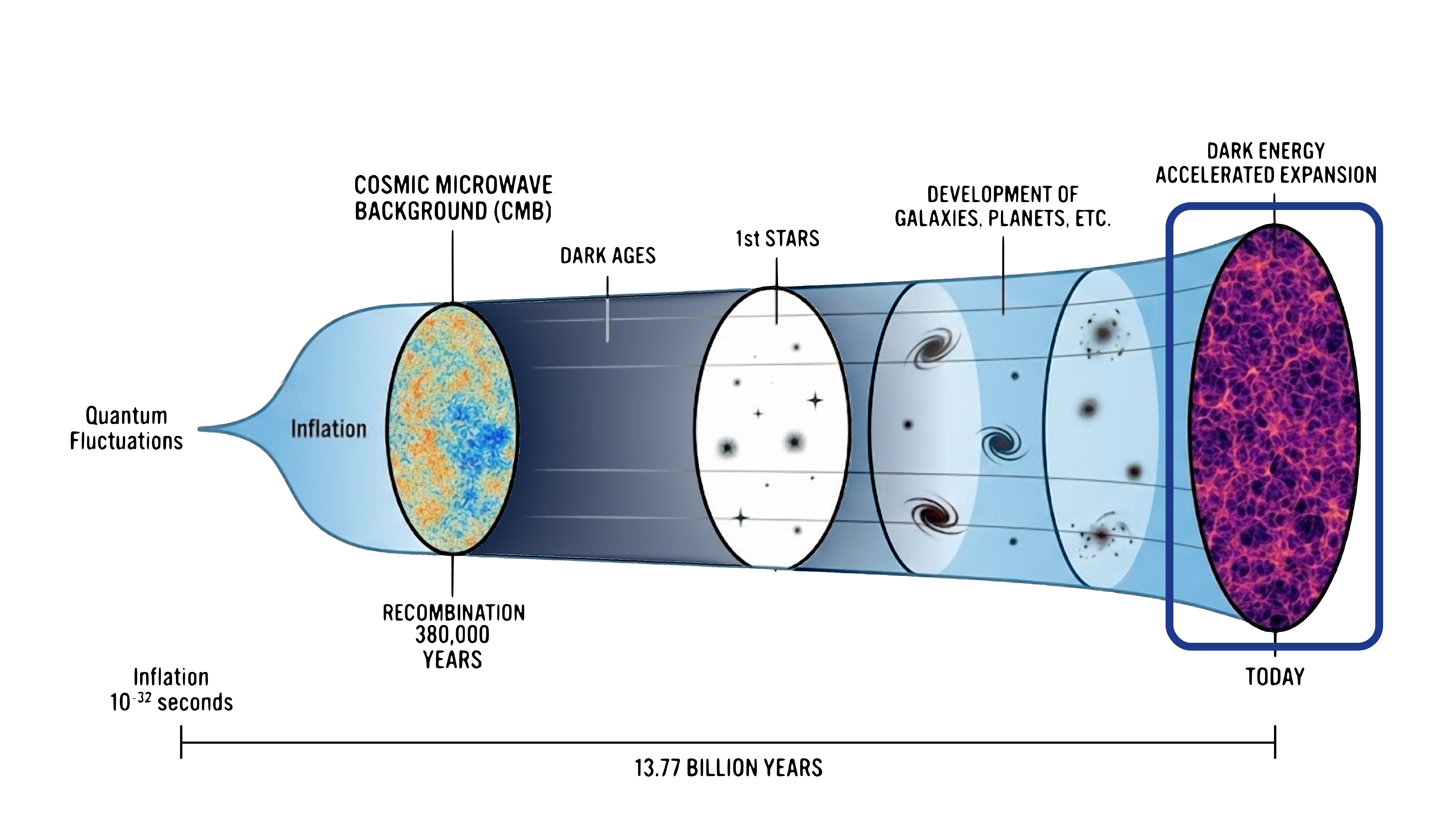
The early Universe
horizon
Credit: NASA / WMAP Science Team
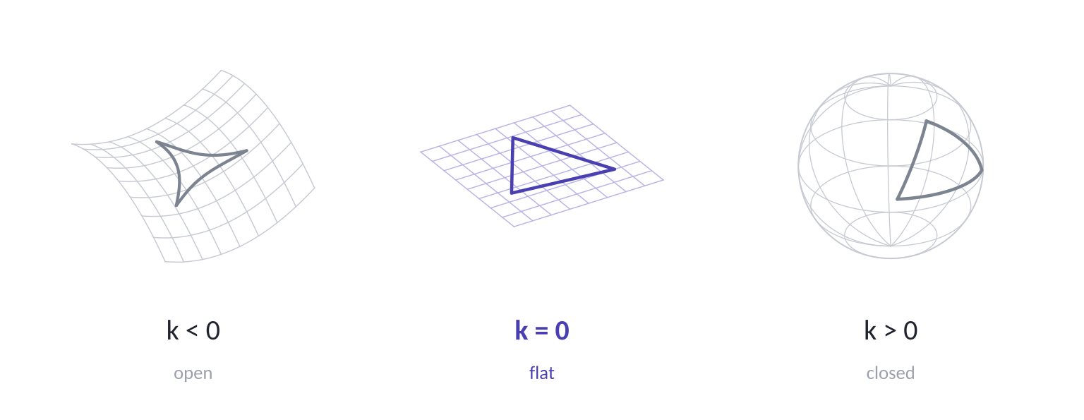
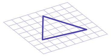
flatness
+ origin of inhomogeneities
+ magnetic monopole problem
The late Universe
dark energy
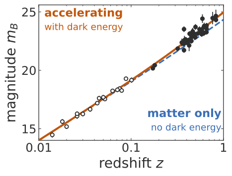
Data: Perlmutter et al. (1999)
Nobel
2011
dark matter
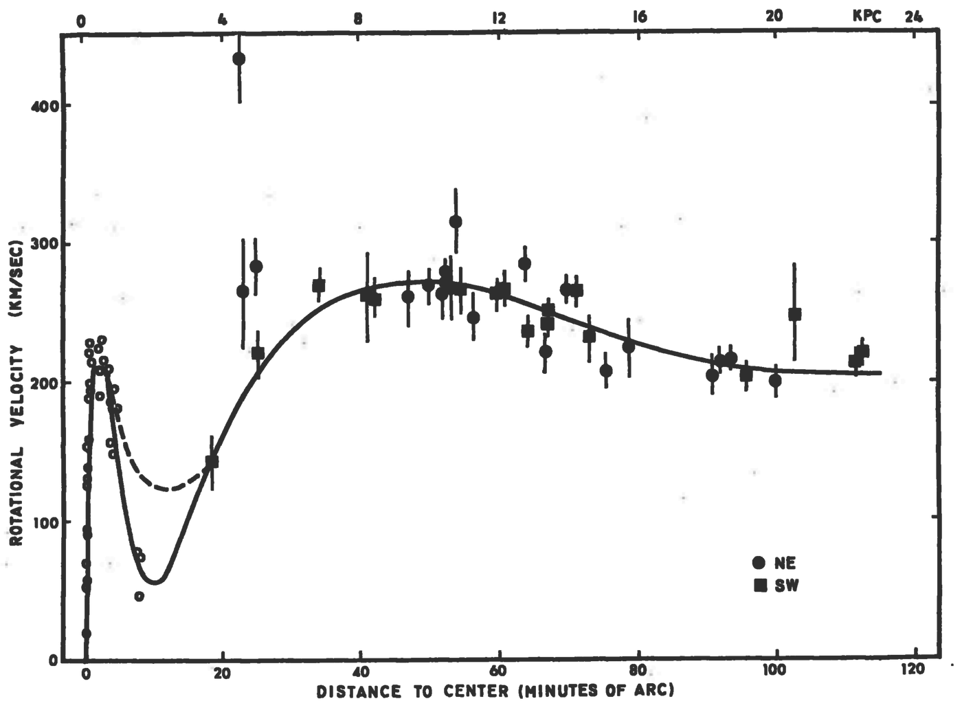
Rubin & Ford (1970), Fig. 9 (M31)
Kabalan et al. (2026) · submitted to RASTI
Kabalan et al. (2026b) · accepted to JOSS
Kabalan et al. (2026c) · in prep. for JCAP
Kabalan et al. (2026) · submitted to RASTI
Kabalan et al. (2026b) · accepted to JOSS
Kabalan et al. (2026c) · in prep. for JCAP
The early Universe
horizon
flatness
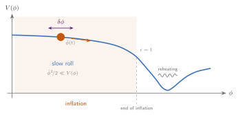
\[ r \equiv \frac{A_t}{A_s} \;\propto\; E_\mathrm{inf}^4 \]
The tensor-to-scalar ratio determines the energy scale of inflation
Primordial Gravitational Waves leave a unique imprint in the CMB polarisation
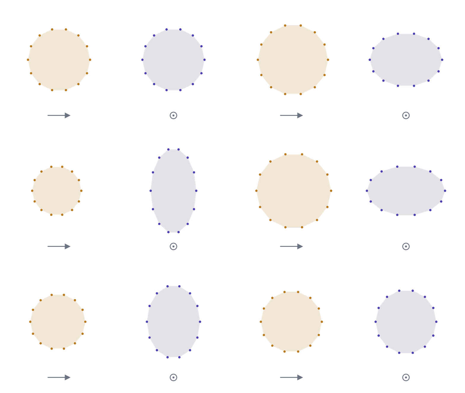
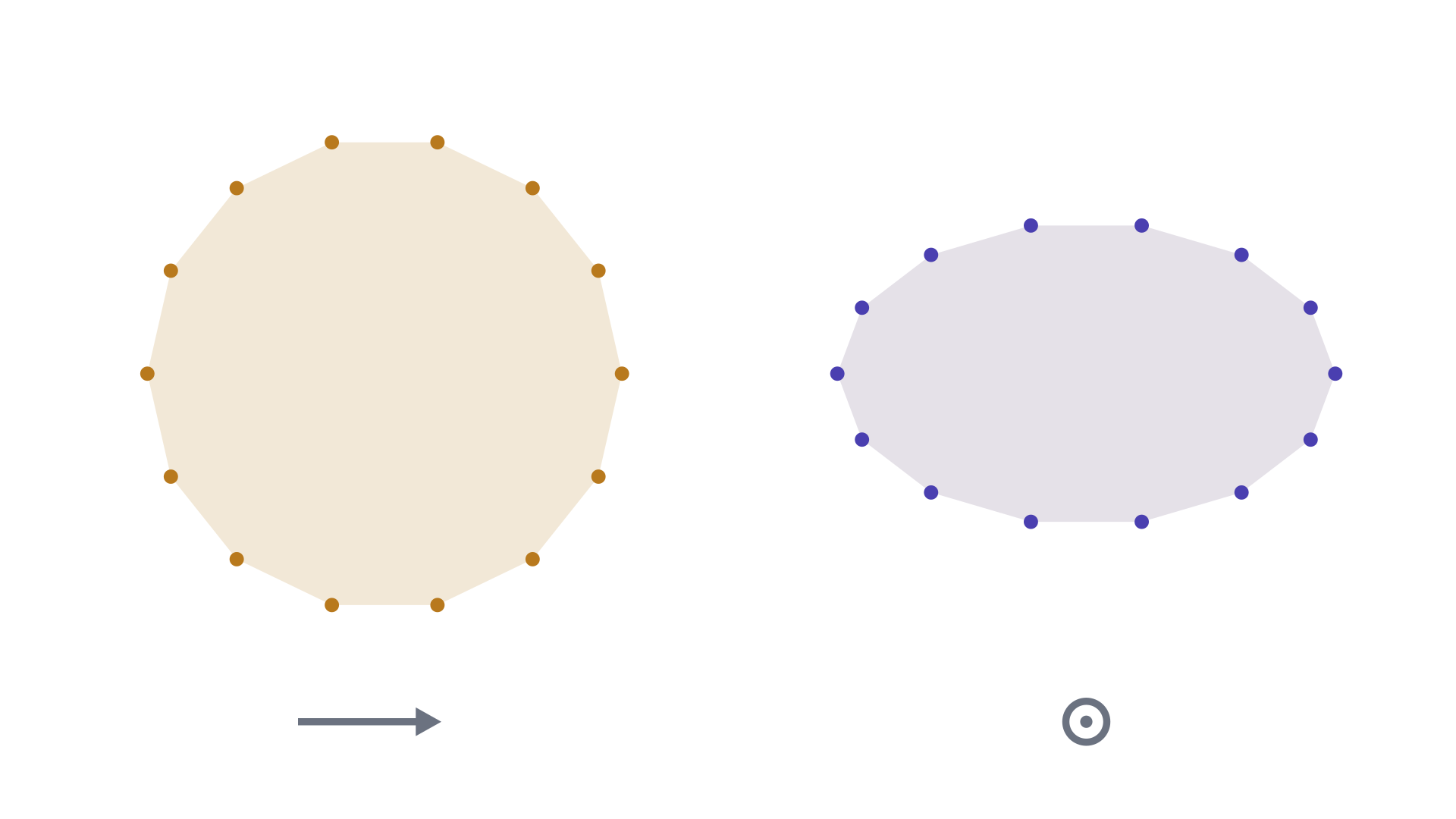
The last scattering surface
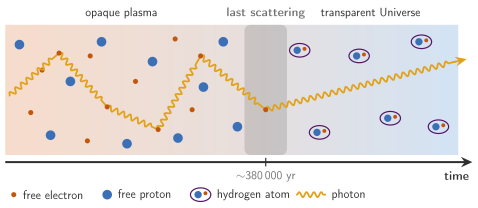
Adapted from: Yacine Ali-Haïmoud (NYU, 2019)
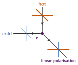
Adapted from: Hu & White (1997)
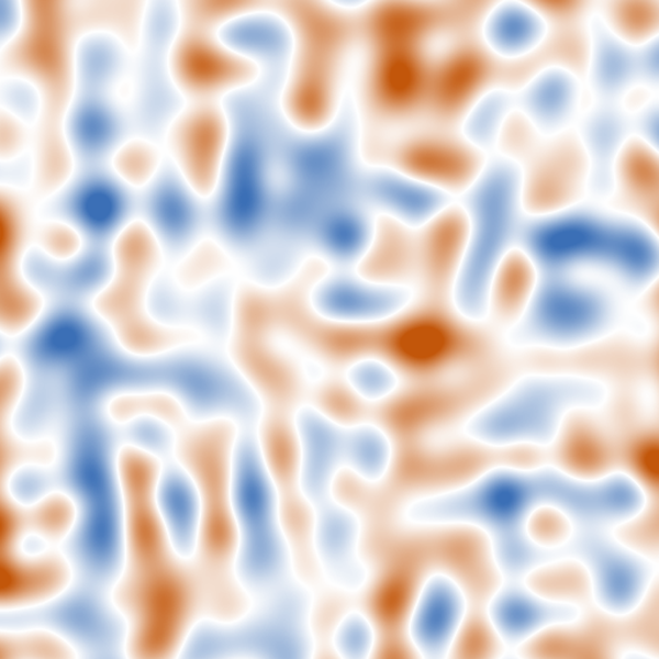 \(Q\)
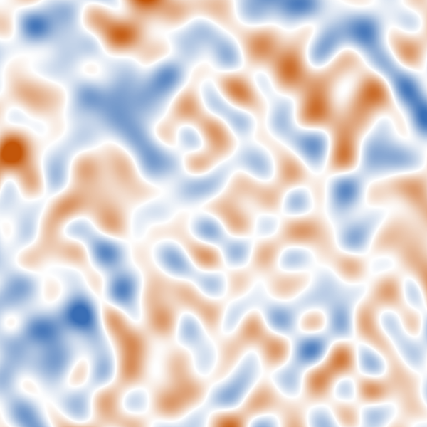 \(U\)
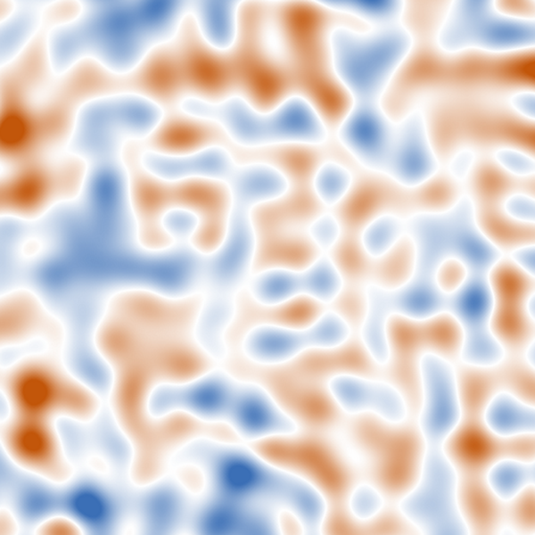 \(Q\)\(U\)
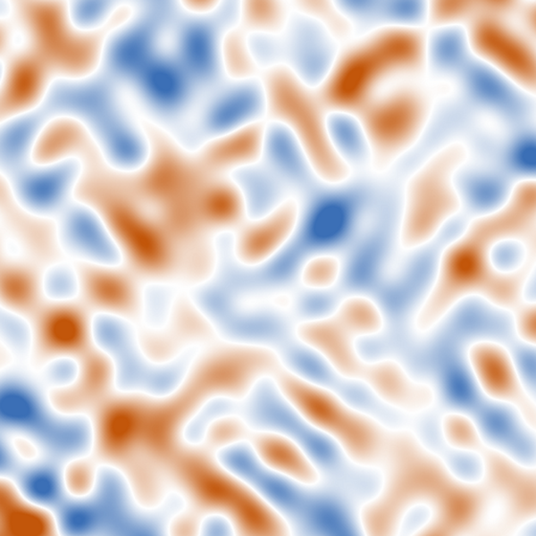 \(U\)\(-Q\)
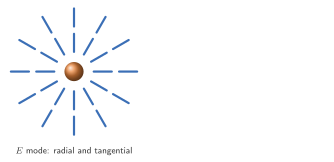
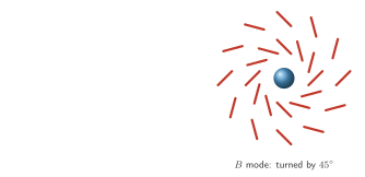
\(Q\) and \(U\) depend on the reference frame: turning it by \(45^\circ\) swaps them, \(Q'\) \(=\) \(U\) and \(U'\) \(= -\)\(Q\)
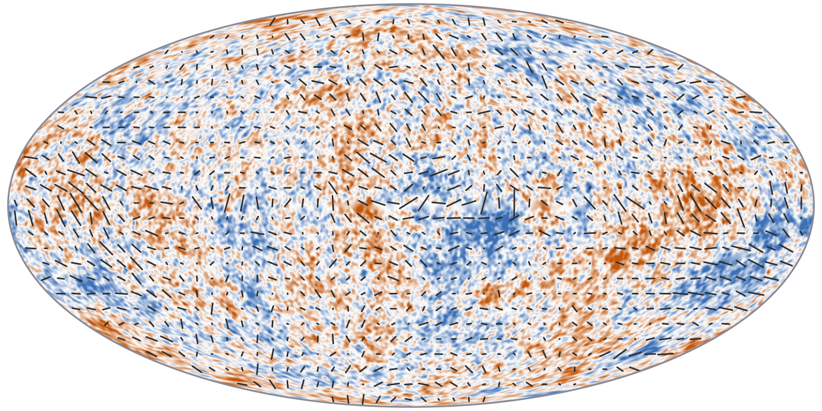
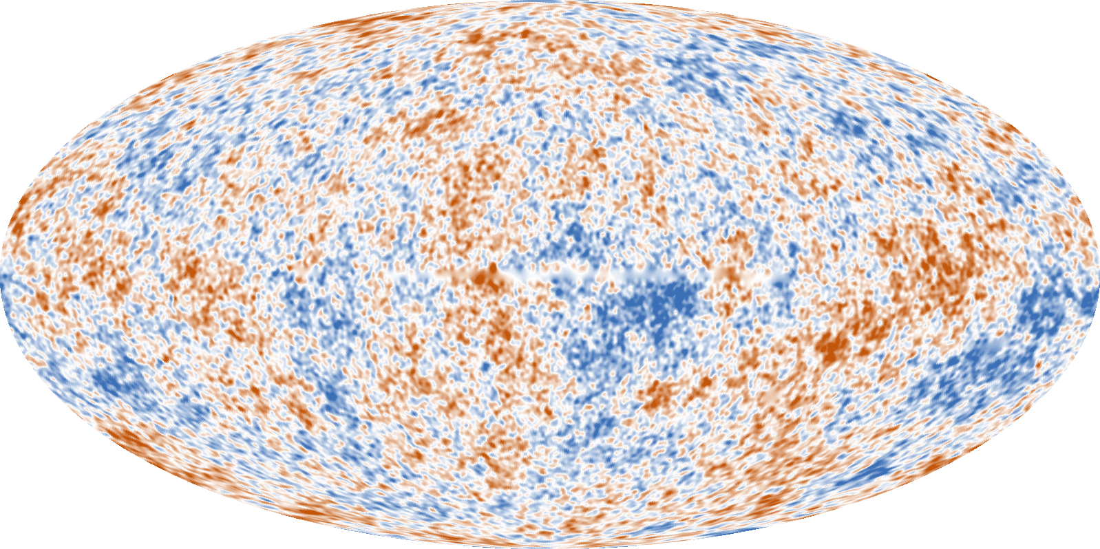
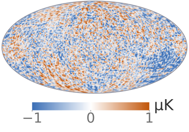
Planck 2018 SMICA: temperature (colour), polarisation (sticks)


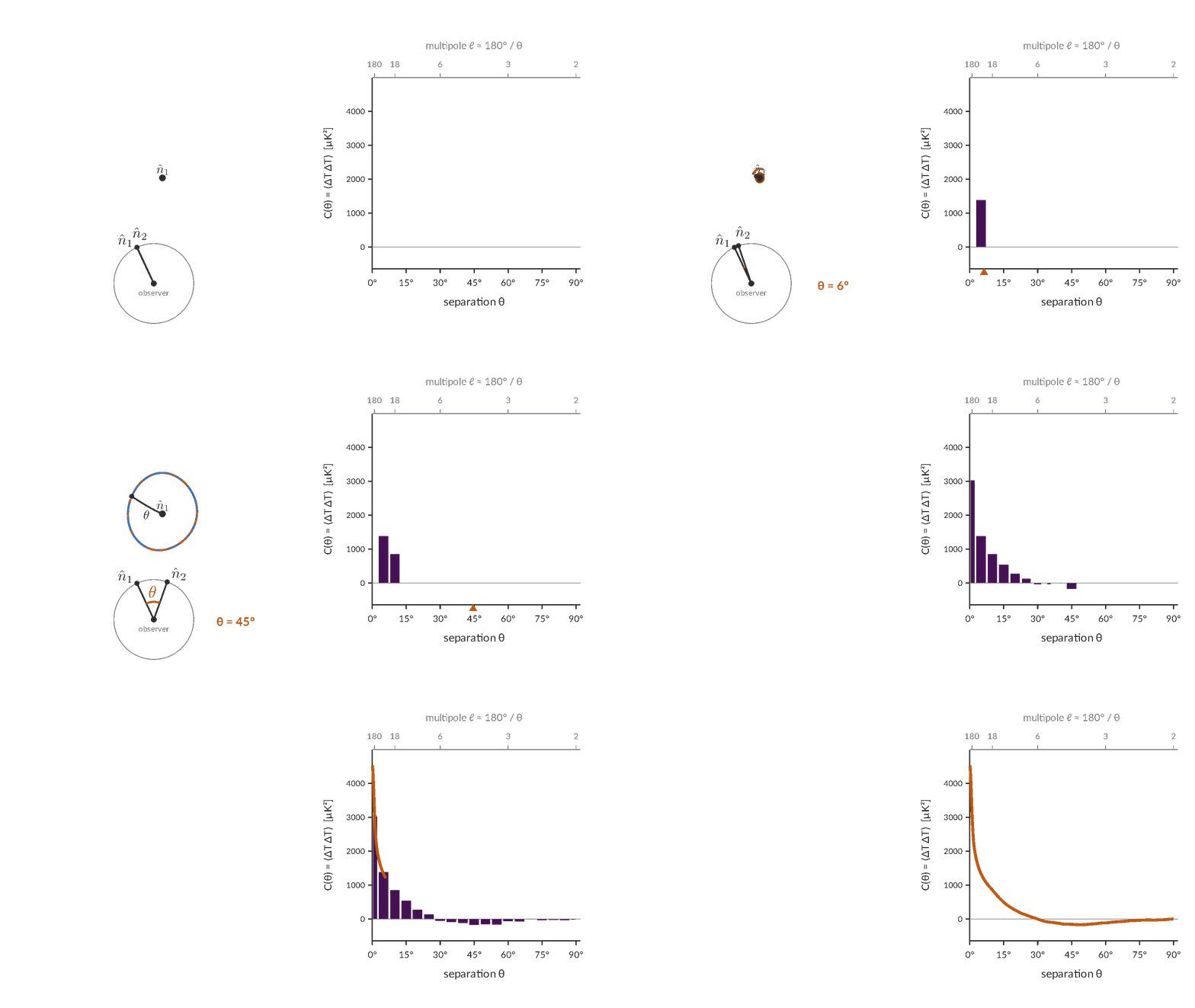
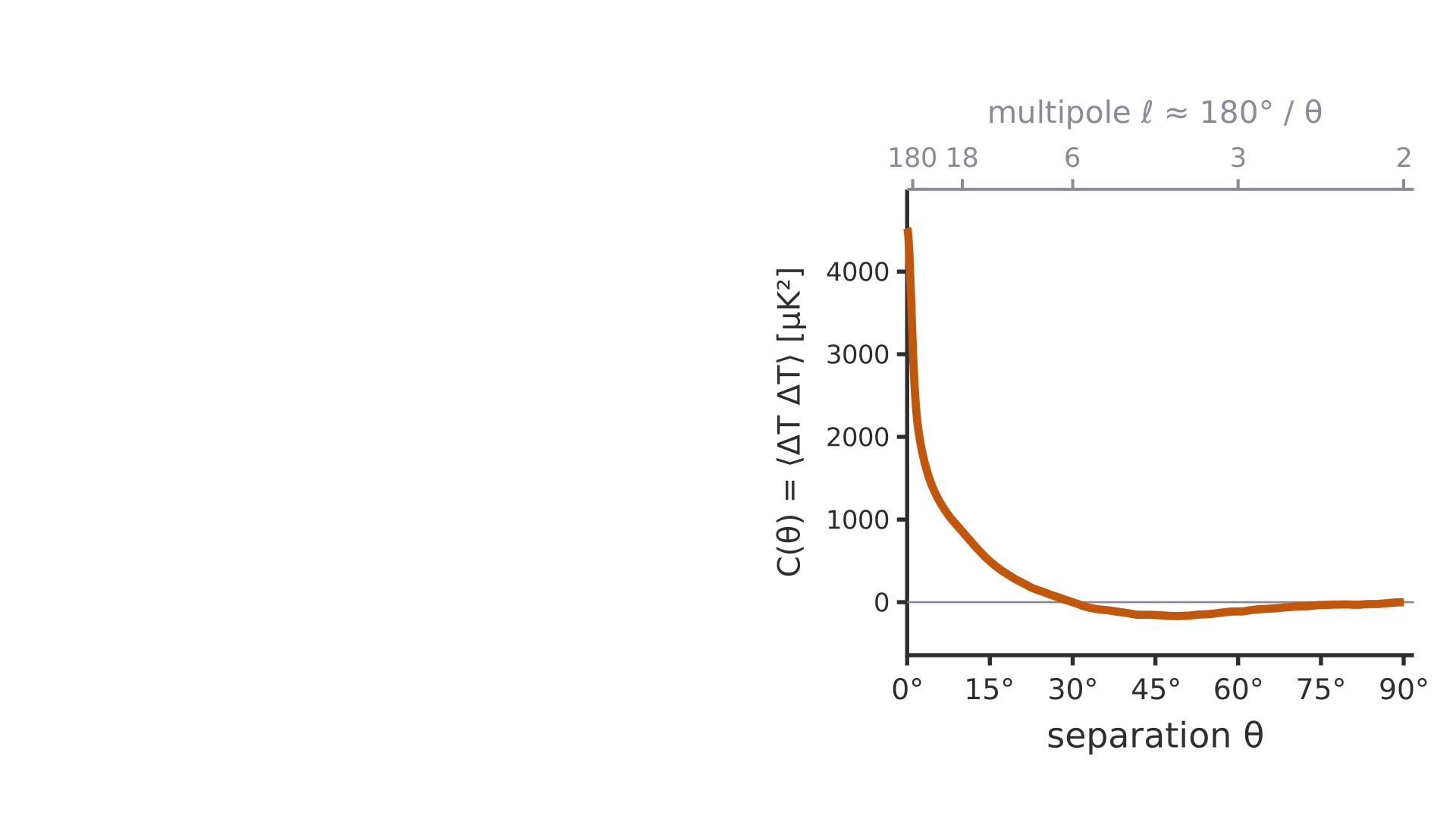
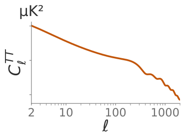
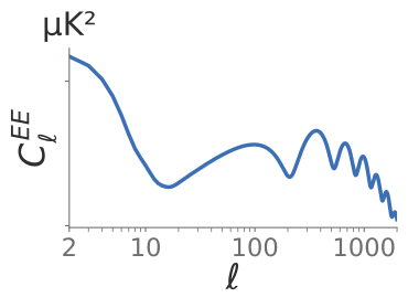
\(C(\theta) = \langle \Delta T(\hat n_1)\,\Delta T(\hat n_2)\rangle\) over all pairs at separation \(\theta\): its expansion in Legendre polynomials gives the \(C_\ell\)
Planck 2018 SMICA temperature map · smoothed to 1° FWHM
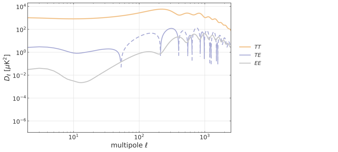
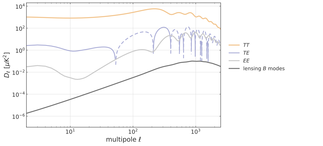
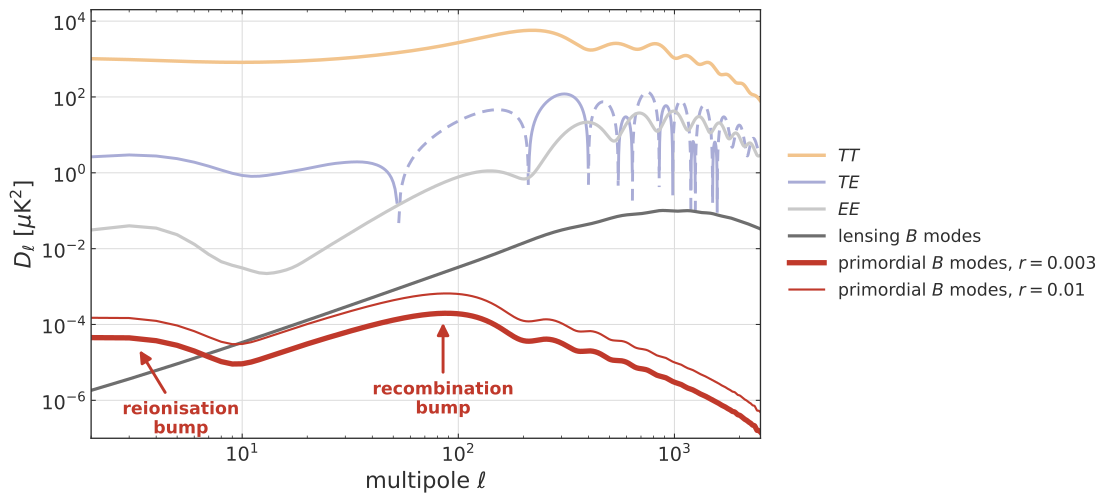
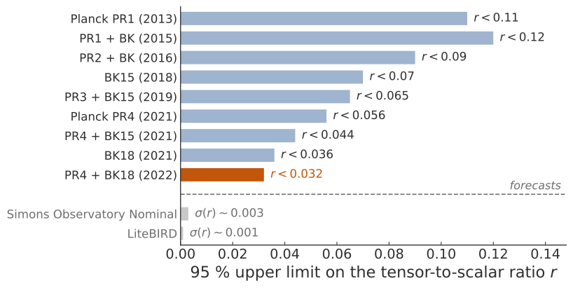
Tristram et al. (2022); Simons Observatory (Ade et al. 2019); LiteBIRD Collaboration (2023)
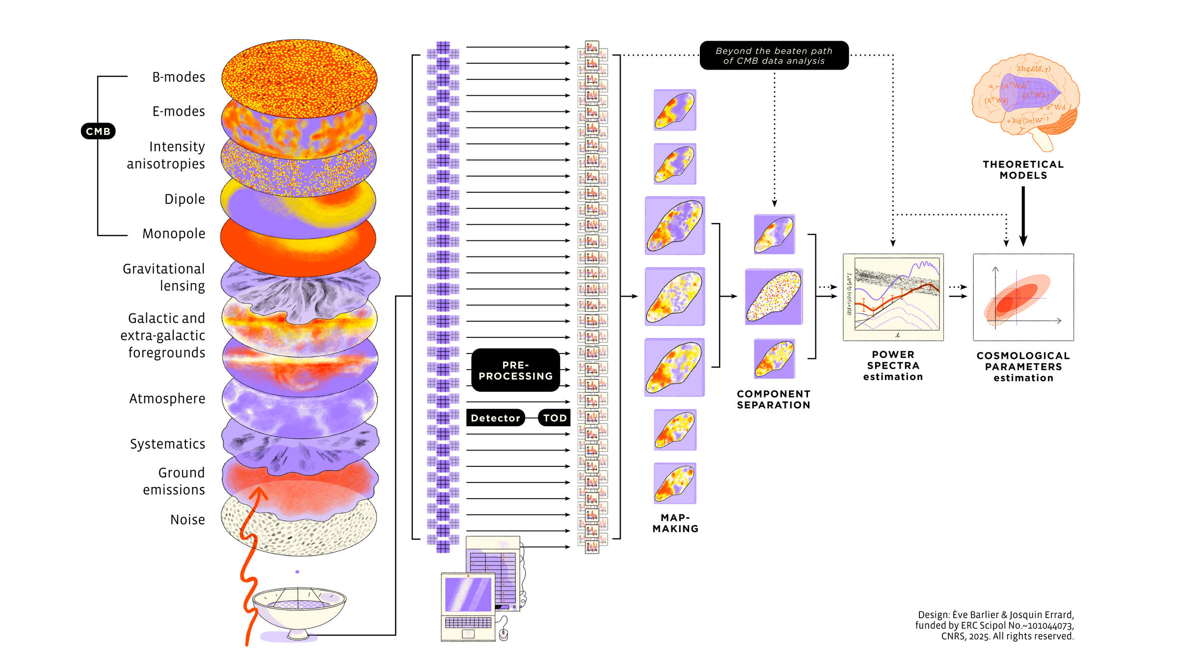
My contribution
Kabalan et al. (2026) · submitted to RASTI
Kabalan et al. (2026b) · accepted to JOSS
Kabalan et al. (2026c) · in prep. for JCAP
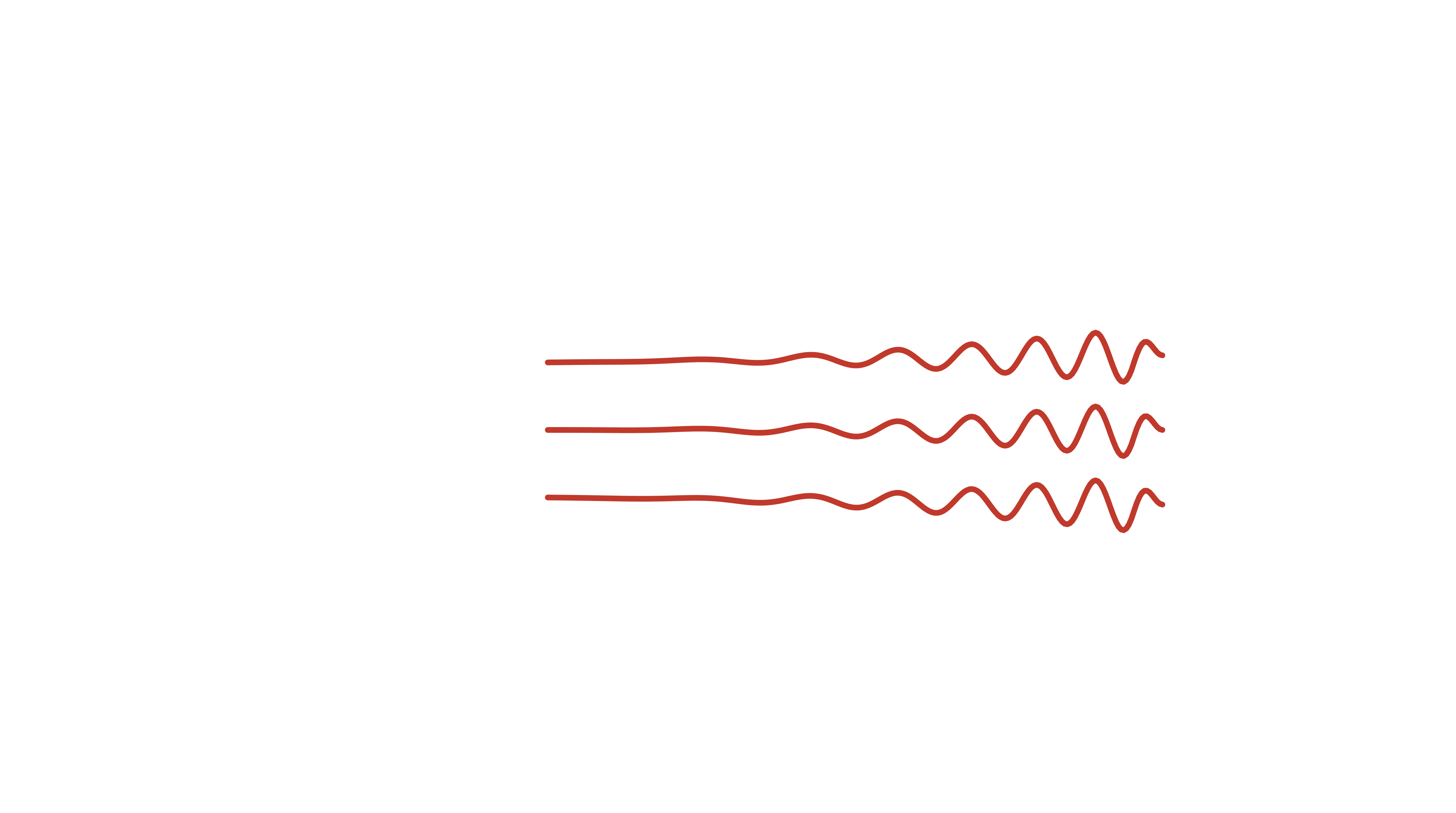
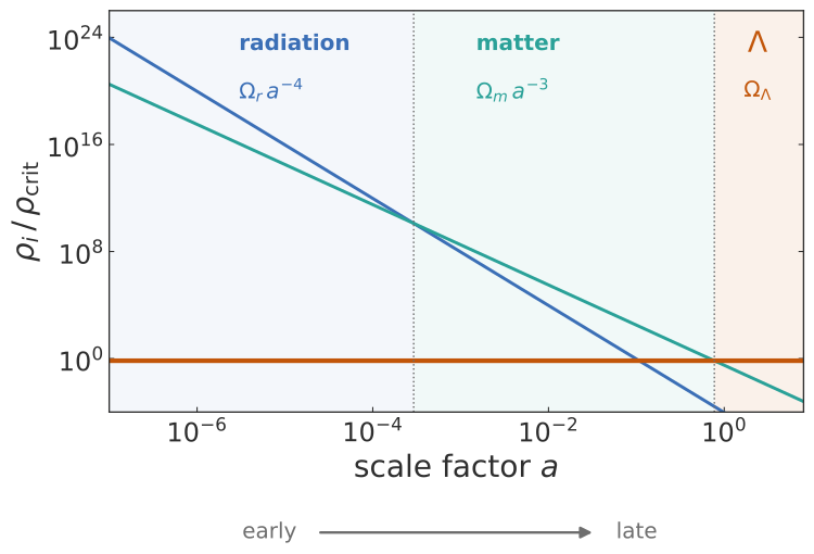
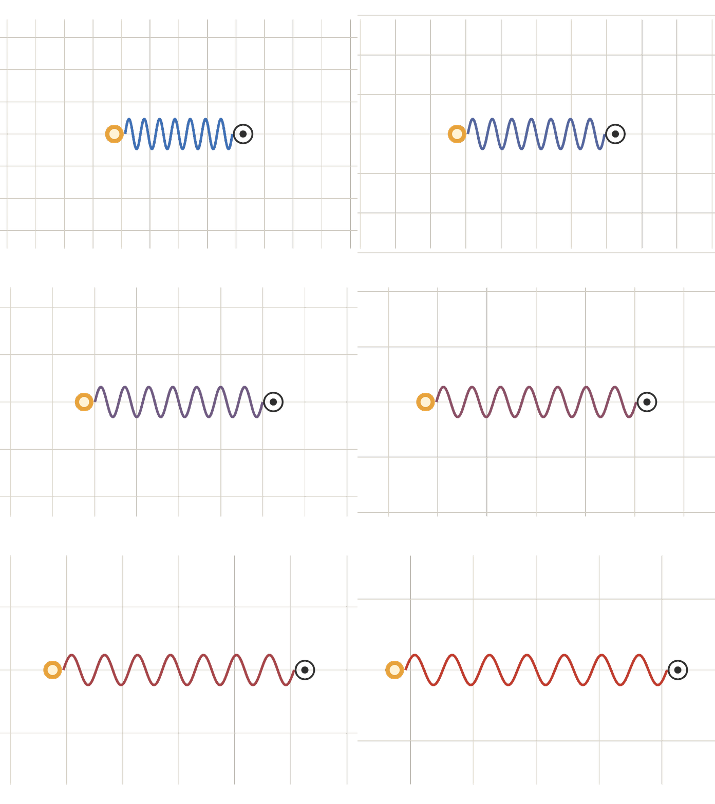
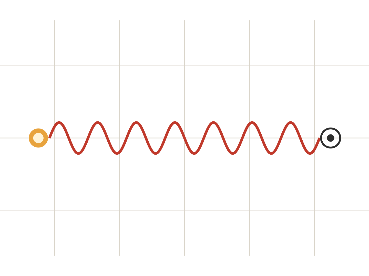
redshift \(1 + z = \dfrac{\lambda_\mathrm{obs}}{\lambda_\mathrm{emit}} = \dfrac{1}{a}\)
scale factor \(a(t),\qquad a_0 = 1,\qquad H = \dot a / a\)
comoving distance \(\chi(z) = \displaystyle\int_0^z \frac{c\,dz'}{H(z')}\)
expansion rate \(H(z) = H_0\sqrt{\Omega_r(1+z)^4 + \Omega_m(1+z)^3 + \Omega_\Lambda}\)
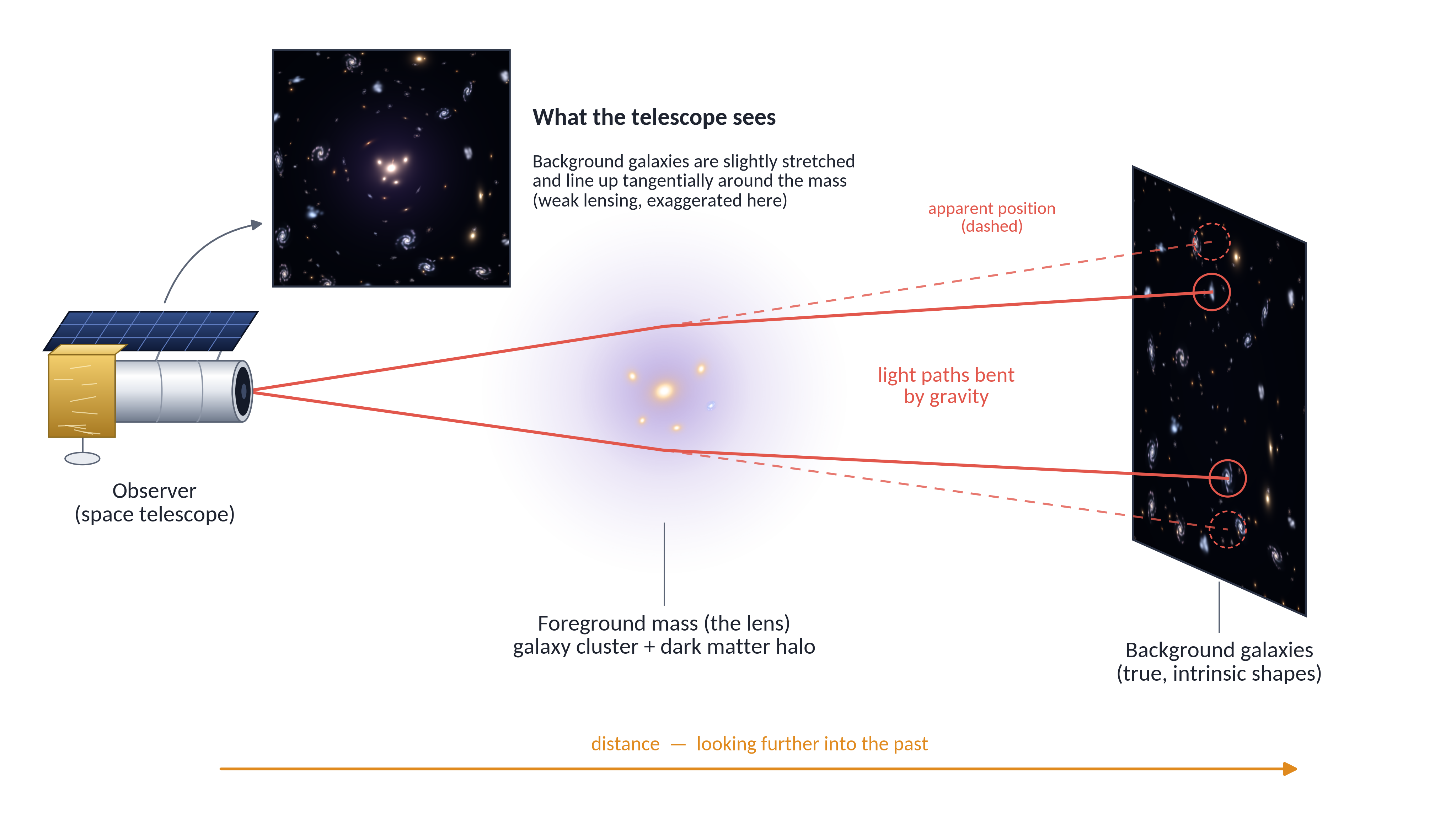
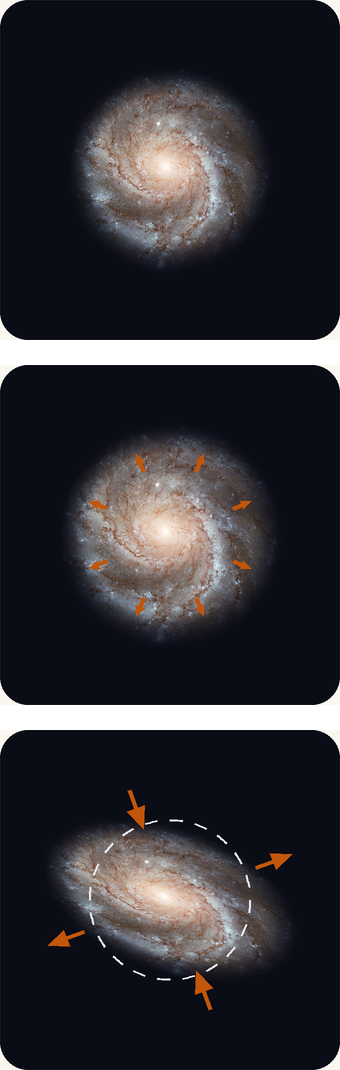
Matter along the line of sight bends light: every background galaxy is slightly distorted
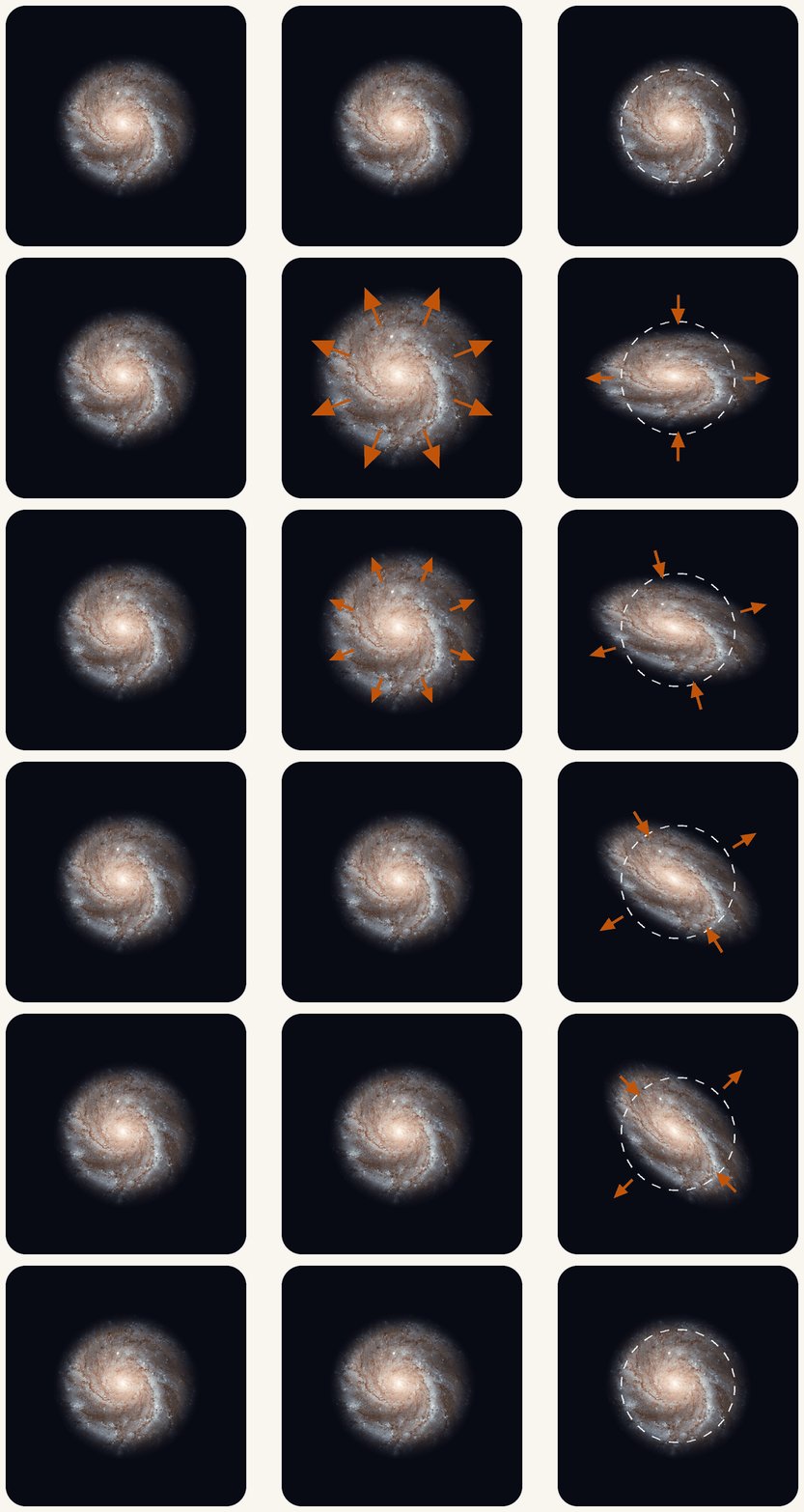
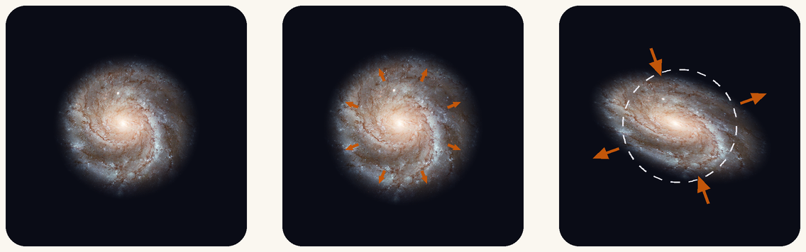
galaxy
convergence \(\kappa\) (spin 0)
shear \(\gamma_1, \gamma_2\) (spin 2)
M101: NASA / ESA / Hubble (STScI-PRC2006-10a)
\[ \mathbf{A} = \begin{pmatrix} 1-\kappa-\gamma_1 & -\gamma_2 \\ -\gamma_2 & 1-\kappa+\gamma_1 \end{pmatrix} \]
Matter deforms galaxies through weak lensing, by a spin-0 field, the convergence \(\kappa\), and a spin-2 field, the two components of the shear \(\gamma\)
Distant galaxies lensed by the cosmic web
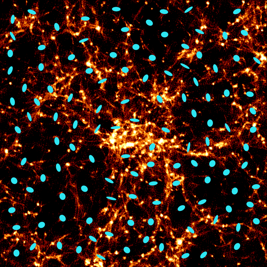
After Mandelbaum (2018), arXiv:1710.03235, Fig. 1 (image: CFHT) · shell of this work’s 3072³ run, z = 0.36
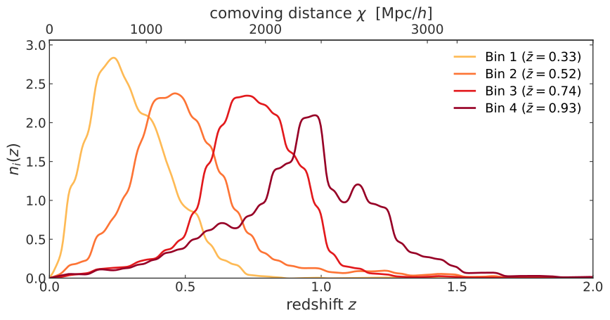
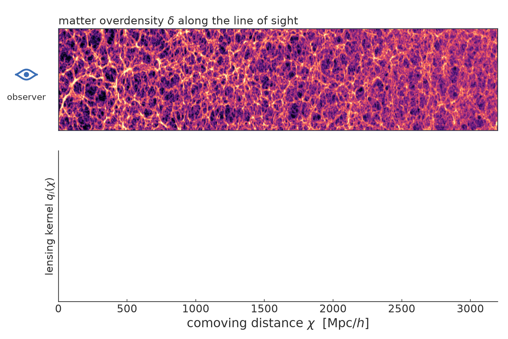
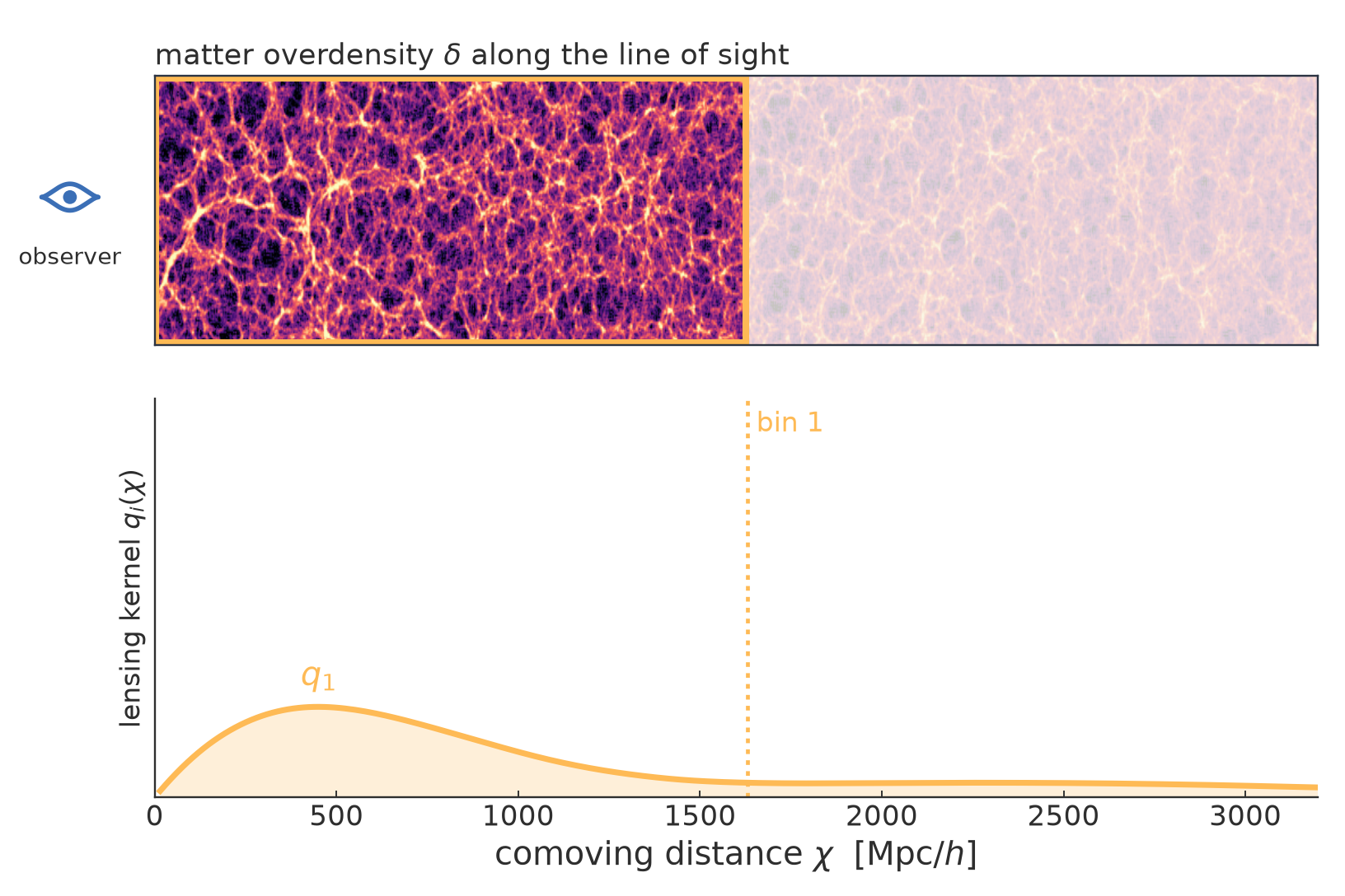
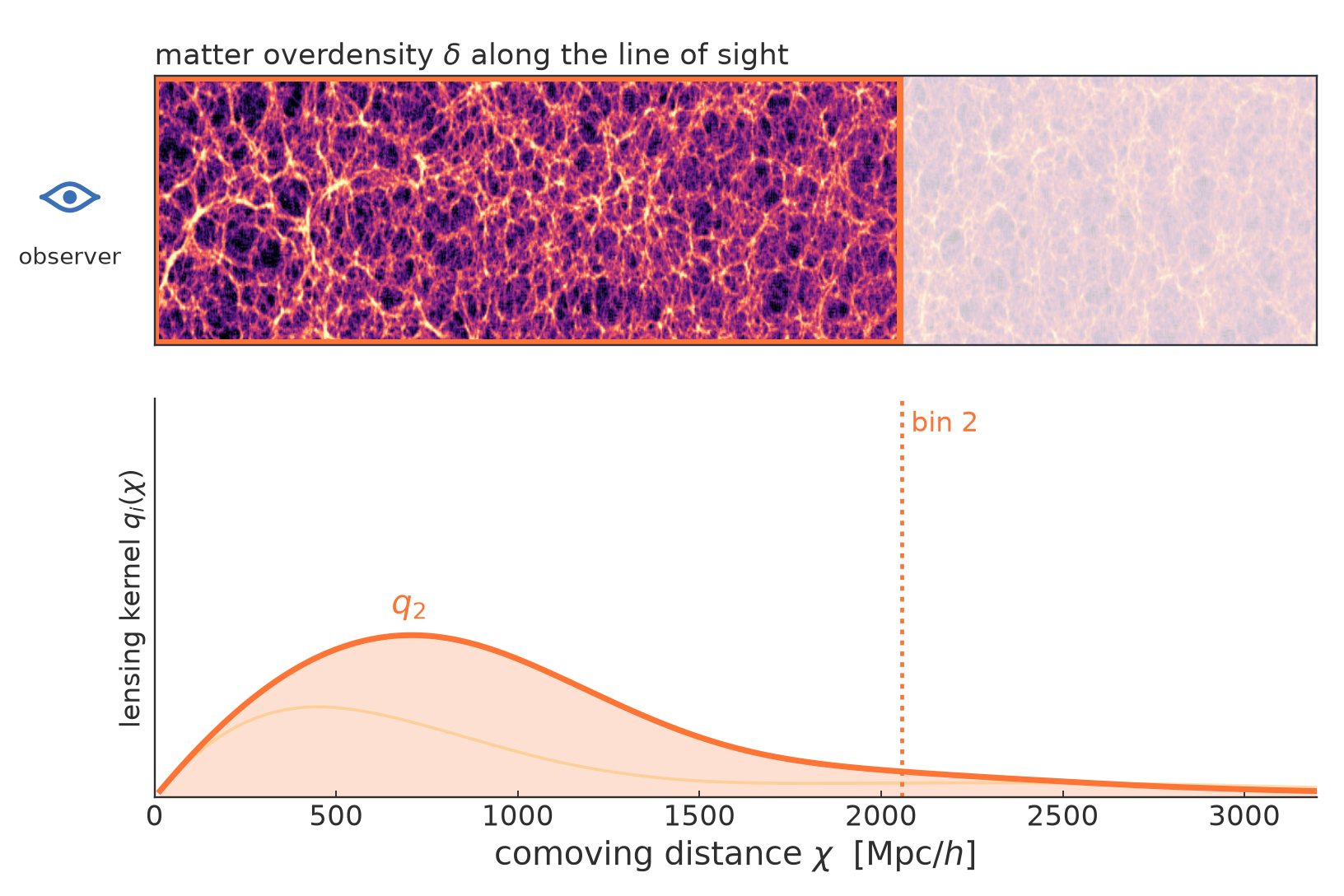
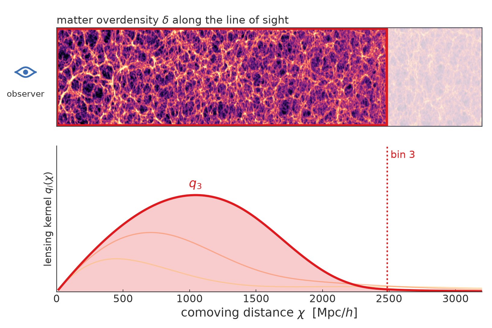
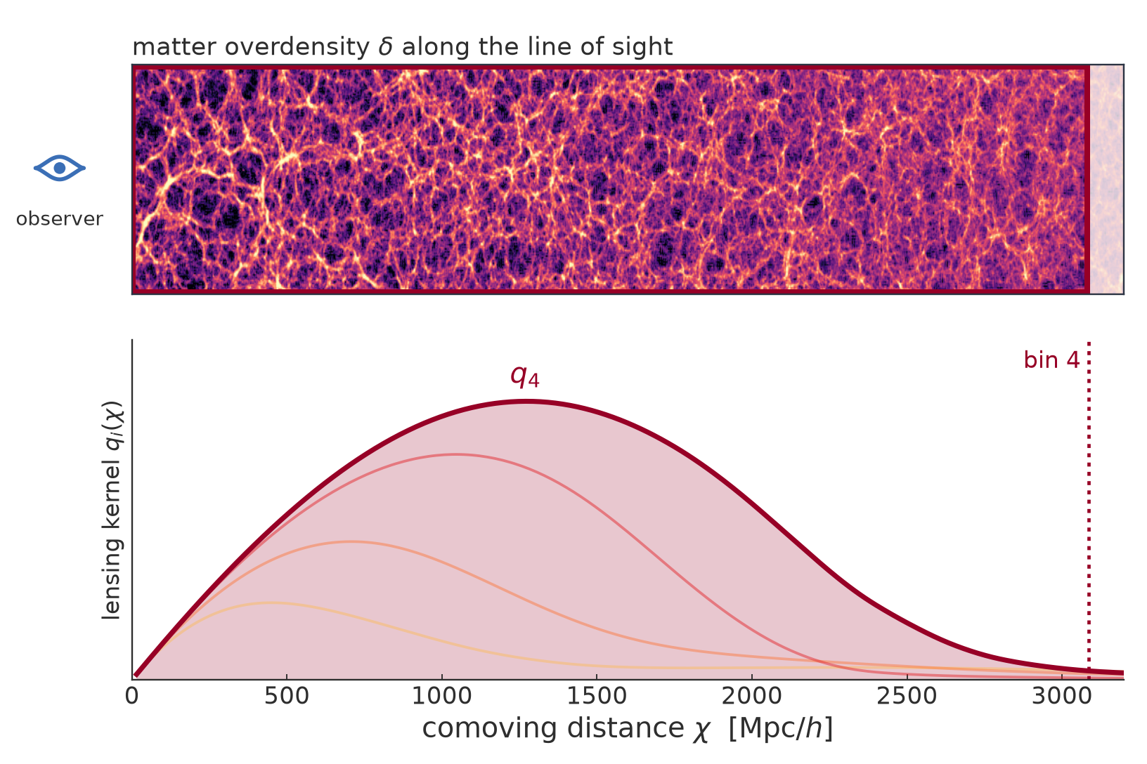
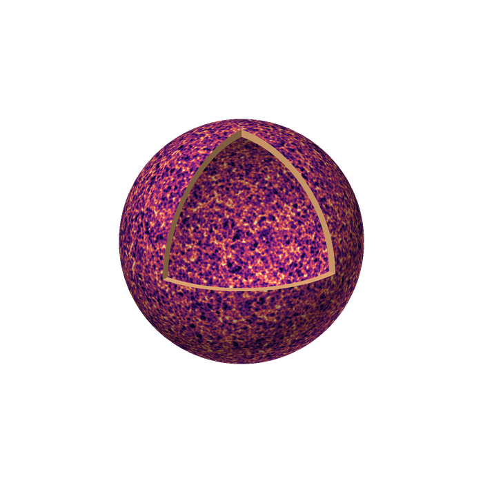
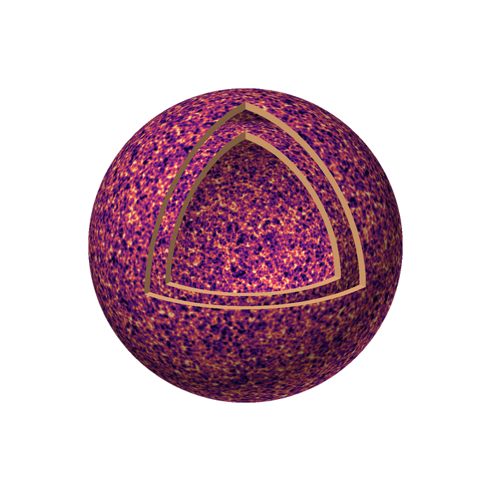
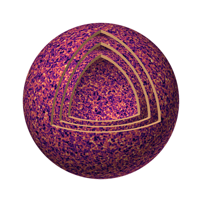
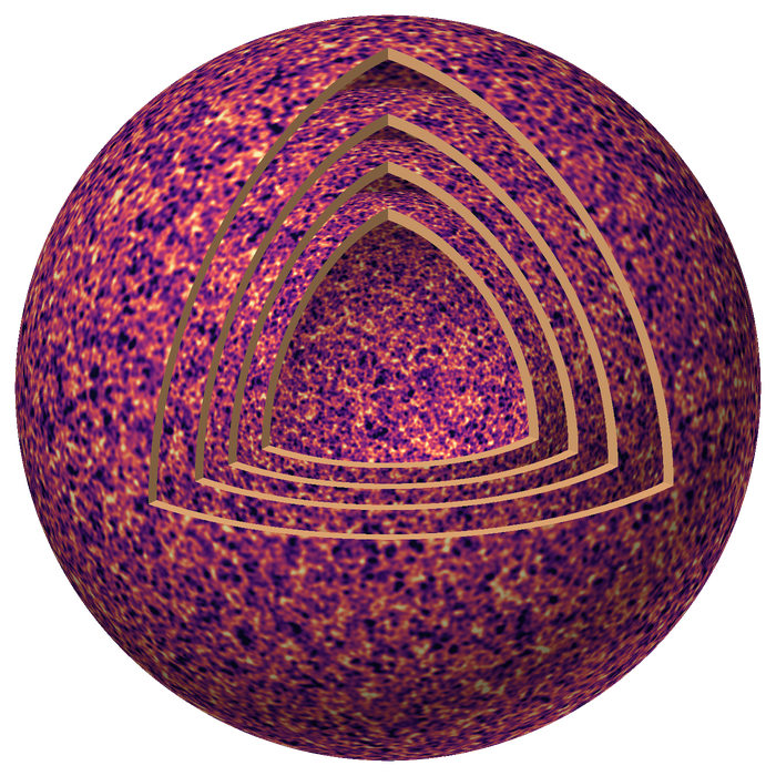
\[\kappa_i(\hat{\mathbf n}) = \int_0^{\chi_H} q_i(\chi)\,\delta(\chi\hat{\mathbf n},\chi)\,\mathrm{d}\chi\]
Shell rendering inspired by GLASS (Tessore et al. 2023)
DATA
galaxy
shapes
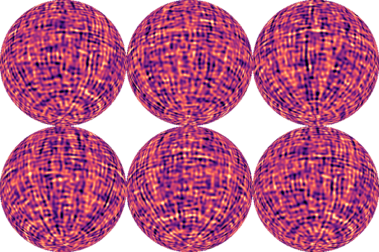
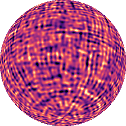
shear \(\gamma_1, \gamma_2\)
Inverse Kaiser–Squires
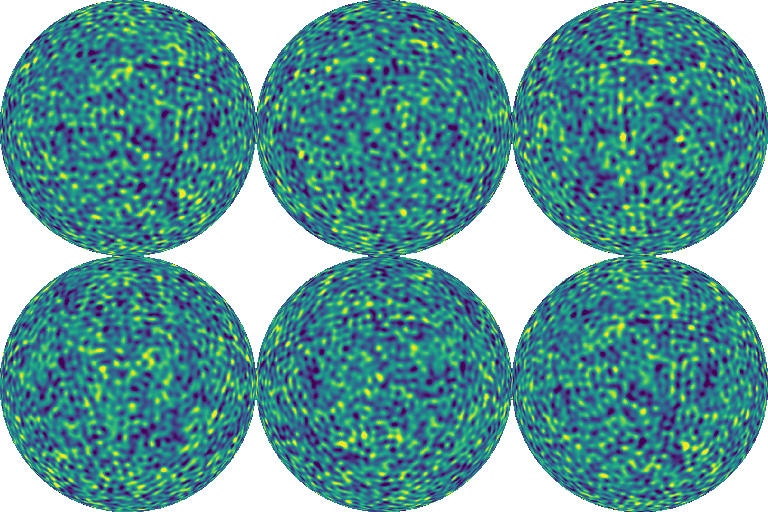
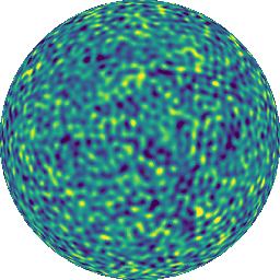
convergence \(\kappa\) per bin
measured
\(\hat C_\ell^{\,ij}\)
THEORY
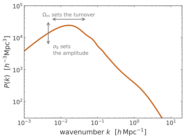
\(\theta = (\Omega_\mathrm{m}, \dots)\)
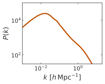
matter spectrum \(P(k, z)\)
Limber, with the lensing kernels \(q_i(\chi)\)
predicted
\(C_\ell^{\,ij}(\theta)\)

compare
↓
infer \(\theta\)
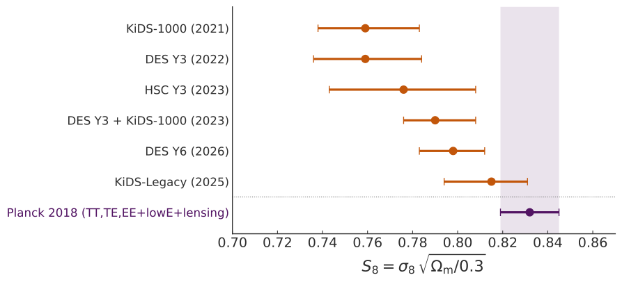
Asgari+21, Secco/Amon+22, Dalal+23, DES & KiDS 2023, Wright+25, DES Y6 2026, Planck 2018 VI
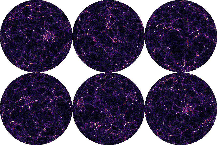
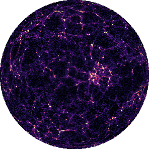
the cosmic web, non-Gaussian
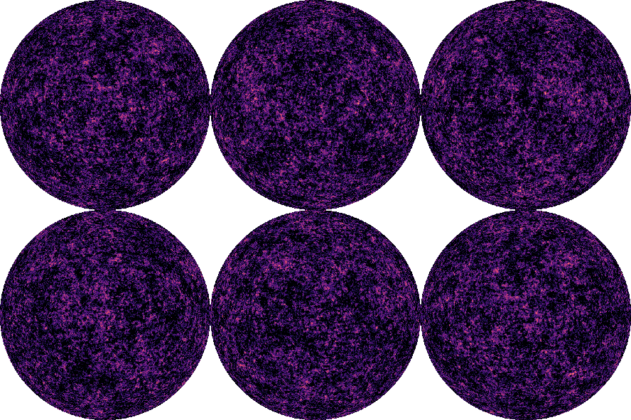
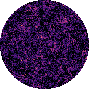
a Gaussian field
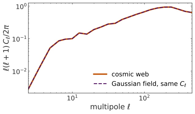
DES Y6 cosmic shear (2026)
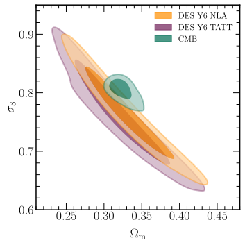
DES Y6 cosmic shear, DES Collaboration (2026), arXiv:2602.10065, Fig. 3 · CMB: Planck 2018, ACT DR6 and SPT-3G, TT+TE+EE+lowE, no lensing
Kabalan et al. (2026) · submitted to RASTI
Kabalan et al. (2026b) · accepted to JOSS
Kabalan et al. (2026c) · in prep. for JCAP
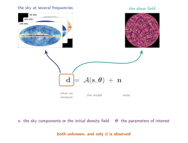
Forward modelling
\[\hat{\mathbf{d}} = \mathcal{A}(\mathbf{s},\boldsymbol\theta)\]
\[-\ln\mathcal{L}(\boldsymbol\theta,\mathbf{s}) \;\propto\; \frac{\lVert \hat{\mathbf{d}} - \mathbf{d} \rVert_2^2}{\sigma^2}\]
Implicit inference
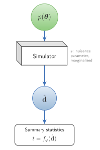
Explicit inference
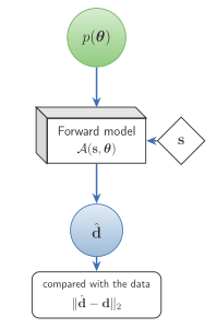
Bayes’ theorem
\[\underbrace{p(\boldsymbol\theta\mid\mathbf{d})}_{\text{posterior}} \;=\; \frac{\overbrace{p(\mathbf{d}\mid\boldsymbol\theta)}^{\text{likelihood}}\;\overbrace{p(\boldsymbol\theta)}^{\text{prior}}}{\underbrace{p(\mathbf{d})}_{\text{evidence}}}\]
\[p(\boldsymbol\theta\mid\mathbf{d}) \;\propto\; p(\mathbf{d}\mid\boldsymbol\theta)\;p(\boldsymbol\theta)\]
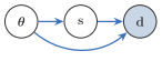
Joint probabilistic modelling
\[p(\boldsymbol\theta,\mathbf{s}\mid\mathbf{d}) \;\propto\; \underbrace{p(\mathbf{d}\mid\mathbf{s},\boldsymbol\theta)}_{\text{likelihood}}\;\underbrace{p(\mathbf{s}\mid\boldsymbol\theta)}_{\text{latent prior}}\;\underbrace{p(\boldsymbol\theta)}_{\text{prior}}\]
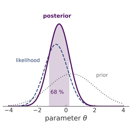
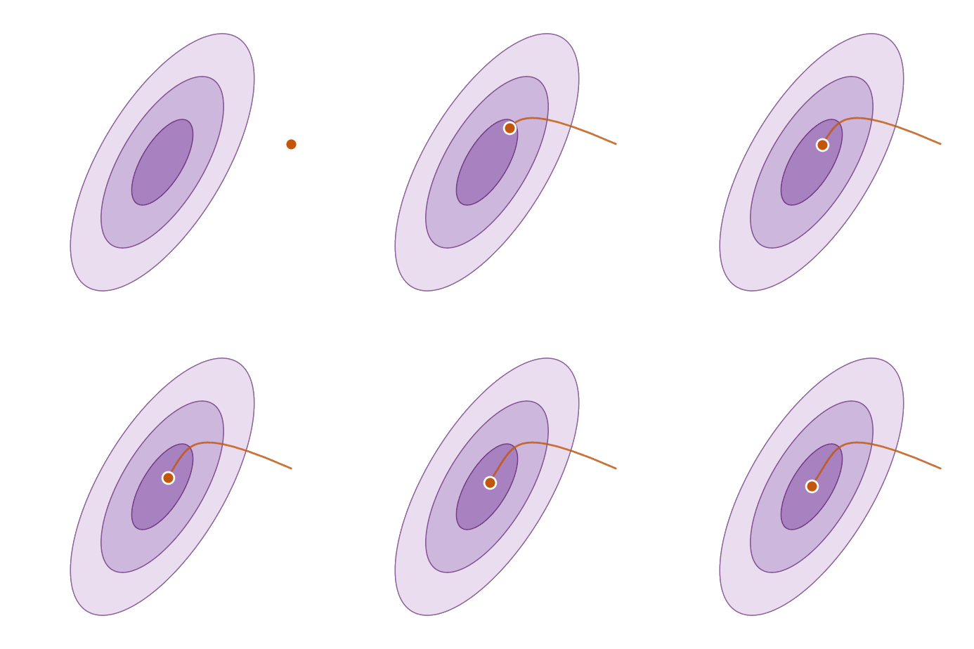
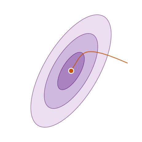
Finding the maximum a posteriori (MAP)
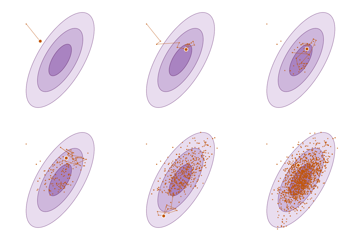
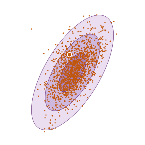
Sampling the full posterior
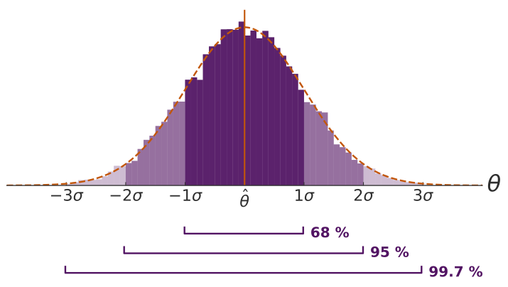
How do we measure how much we trust the result?
Both methods become more efficient with a differentiable likelihood
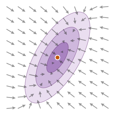
Optimisation: the gradient points to the MAP
\[\boldsymbol\theta_{k+1} = \boldsymbol\theta_k + \eta\,\nabla_{\boldsymbol\theta}\ln p(\boldsymbol\theta\mid\mathbf{d})\]
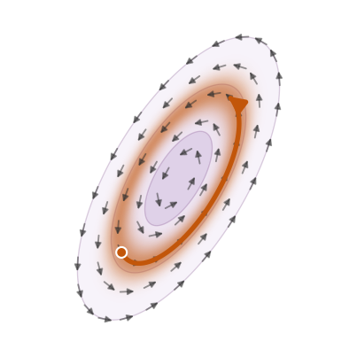
Sampling: Hamiltonian Monte Carlo
\[\dot{\boldsymbol\theta} = \mathbf{p}, \qquad \dot{\mathbf{p}} = \nabla_{\boldsymbol\theta}\ln p(\boldsymbol\theta\mid\mathbf{d})\]
Adapted from Betancourt (2017), arXiv:1701.02434
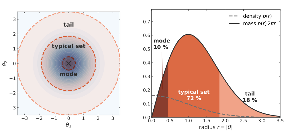
For high-dimensional problems, differentiable likelihoods are required
Likelihood evaluation per independent sample: random walk \(\sim\) \(d\), HMC \(\sim\) \(d^{1/4}\)
Neal (2011); Beskos et al. (2013)



Can better numerical methods improve cosmological pipelines?
Kabalan et al. (2026) · submitted to RASTI
Kabalan et al. (2026b) · accepted to JOSS
Kabalan et al. (2026c) · in prep. for JCAP


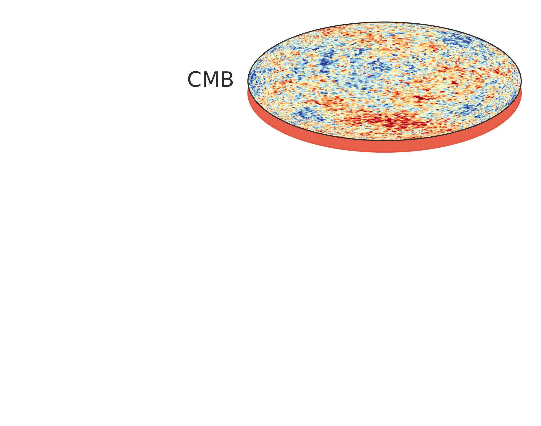
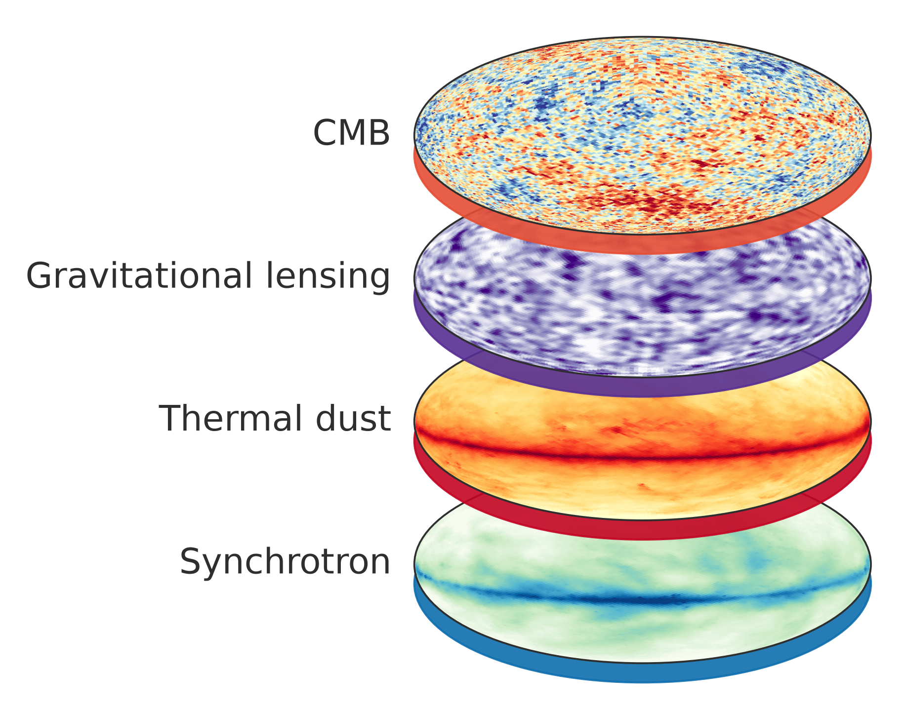
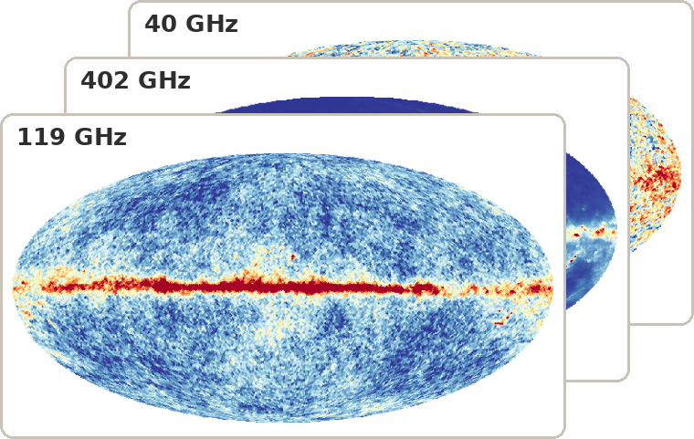
CMB component separation

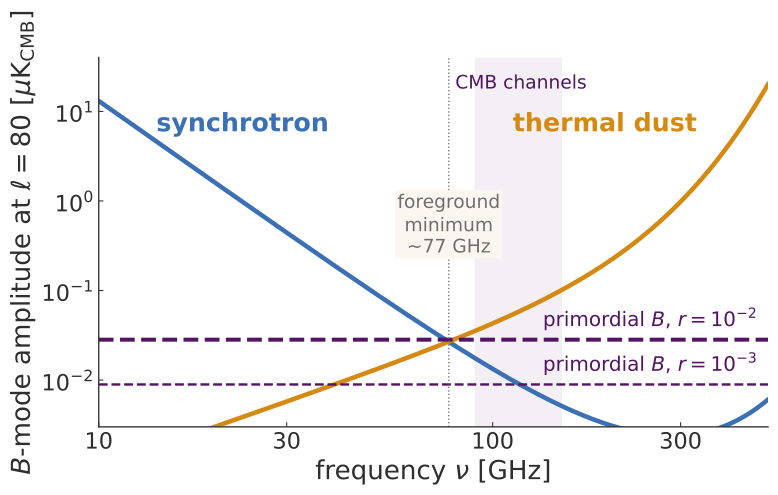
Synchrotron: power law
\[A^{\mathrm{sync}}_\nu({\color{#3b6fb6}\beta_s}) \;\propto\; \left(\frac{\nu}{\nu_0}\right)^{\color{#3b6fb6}\beta_s}\]
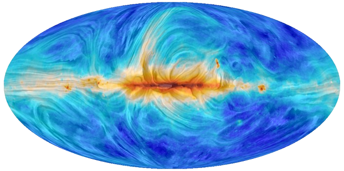
Planck: synchrotron
Dust: modified black body
\[A^{\mathrm{dust}}_\nu({\color{#d68910}\beta_d}, {\color{#d68910}T_d}) \;\propto\; \left(\frac{\nu}{\nu_0}\right)^{{\color{#d68910}\beta_d}+1}\frac{e^{h\nu_0/k{\color{#d68910}T_d}}-1}{e^{h\nu/k{\color{#d68910}T_d}}-1}\]
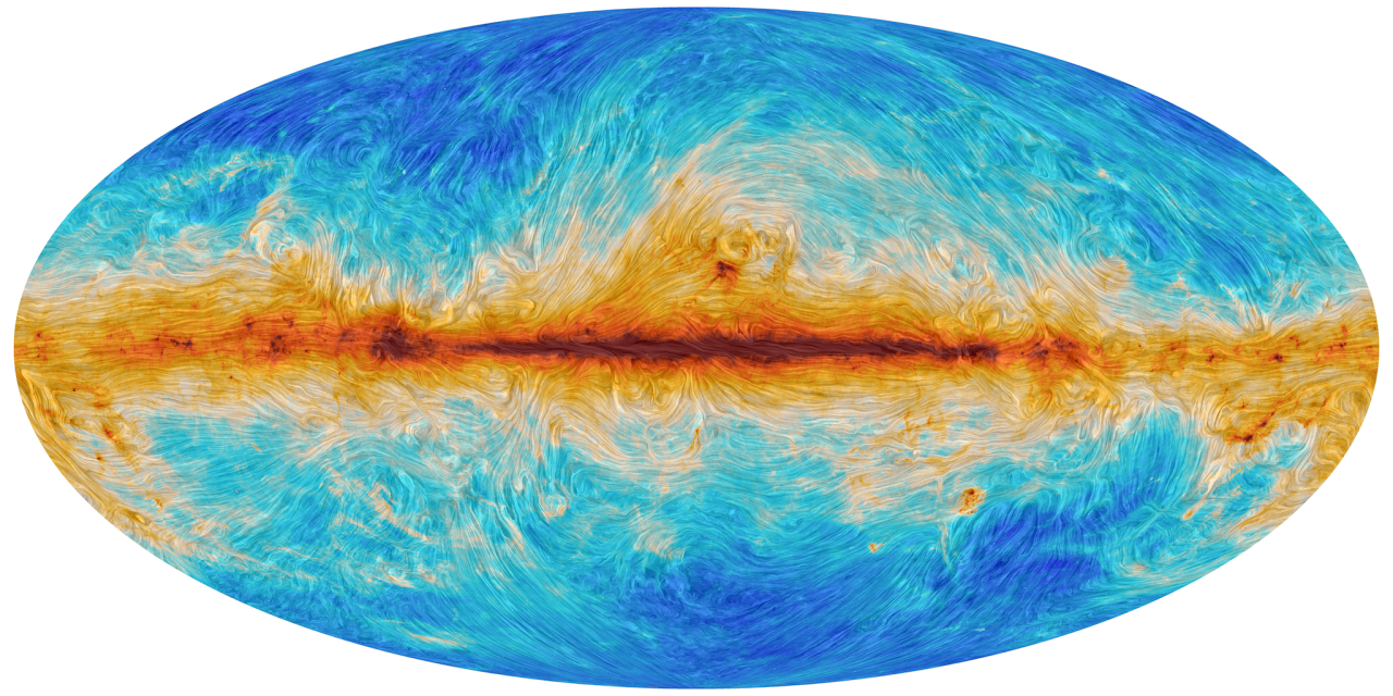
Planck: thermal dust
Rizzieri et al. (2025), arXiv:2510.08534
\[-2\ln\mathcal{L}(\boldsymbol\beta) = -\left(\mathbf{A}^{\top}\mathbf{N}^{-1}\mathbf{d}\right)^{\top}\left(\mathbf{A}^{\top}\mathbf{N}^{-1}\mathbf{A}\right)^{-1}\left(\mathbf{A}^{\top}\mathbf{N}^{-1}\mathbf{d}\right), \qquad \boldsymbol\beta = ({\color{#d68910}\beta_d}, {\color{#d68910}T_d}, {\color{#3b6fb6}\beta_s})\]
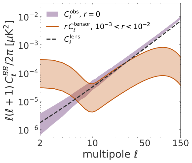
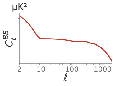
\[C_\ell^{BB,\mathrm{obs}} = C_\ell^{BB,\mathrm{CMB}} + C_\ell^{\mathrm{lens}} + C_\ell^{\mathrm{stat}}\]
\[\text{with}\quad C_\ell^{\mathrm{stat}} = \big\langle C_\ell^{BB,\mathrm{noise}} \big\rangle_n\]
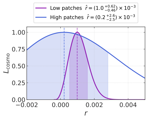
\[C_\ell^{BB,\mathrm{model}}(r) = {\color{#C2560A} r}\,C_\ell^{\mathrm{tensor}} + C_\ell^{\mathrm{lens}} + C_\ell^{\mathrm{stat}}\]
\[-2\ln\mathcal{L}_\mathrm{cosmo}(r) = f_\mathrm{sky}\sum_{\ell}(2\ell+1)\left[\frac{C_\ell^{BB,\mathrm{obs}}}{C_\ell^{BB,\mathrm{model}}(r)} + \ln C_\ell^{BB,\mathrm{model}}(r)\right]\]
synchrotron index \(\beta_s\)
dust index \(\beta_d\)
dust temperature \(T_d\)
SEDs of 300 pixels
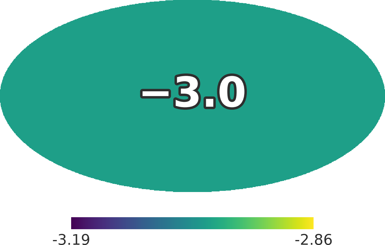
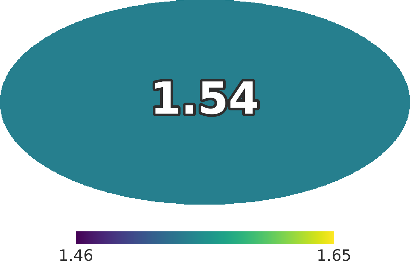
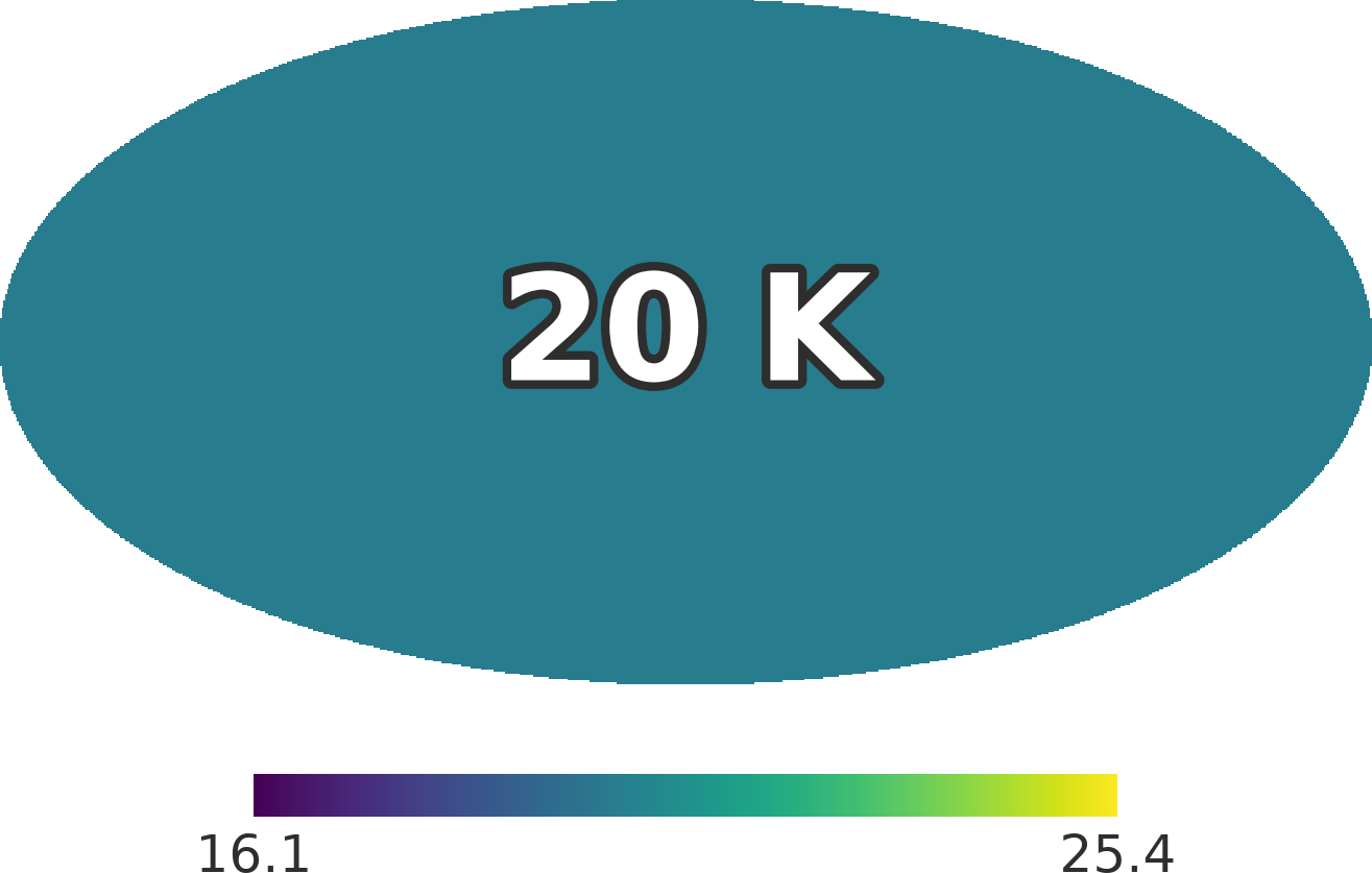
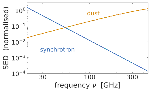
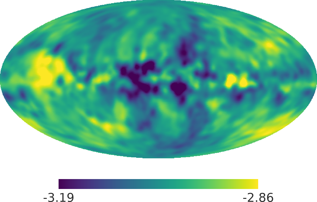
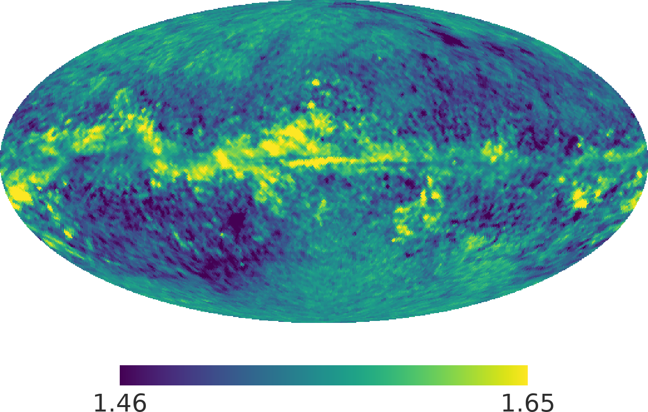
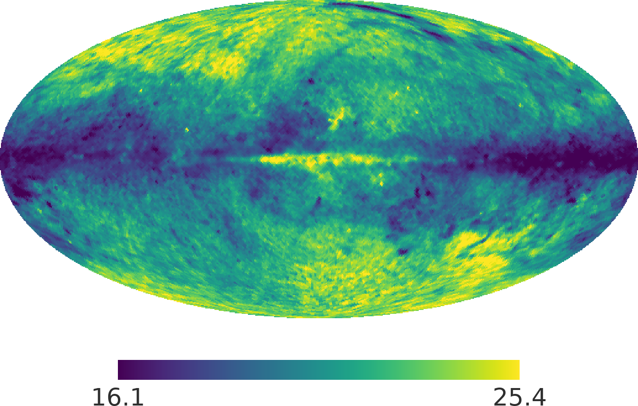
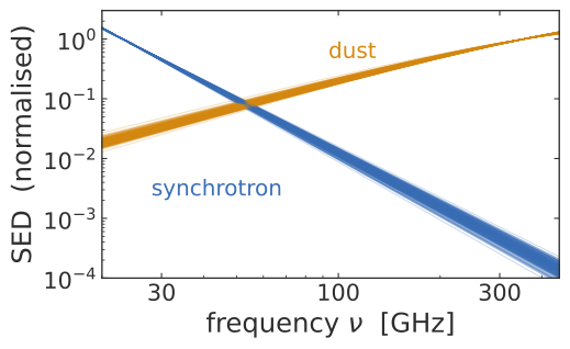
Sky models: PySM (Thorne et al. 2017; Zonca et al. 2021; Pan-Experiment Galactic Science Group 2025)
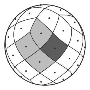
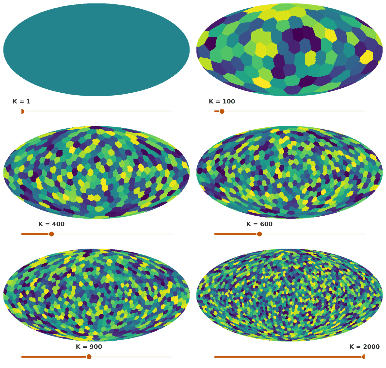
HEALPix

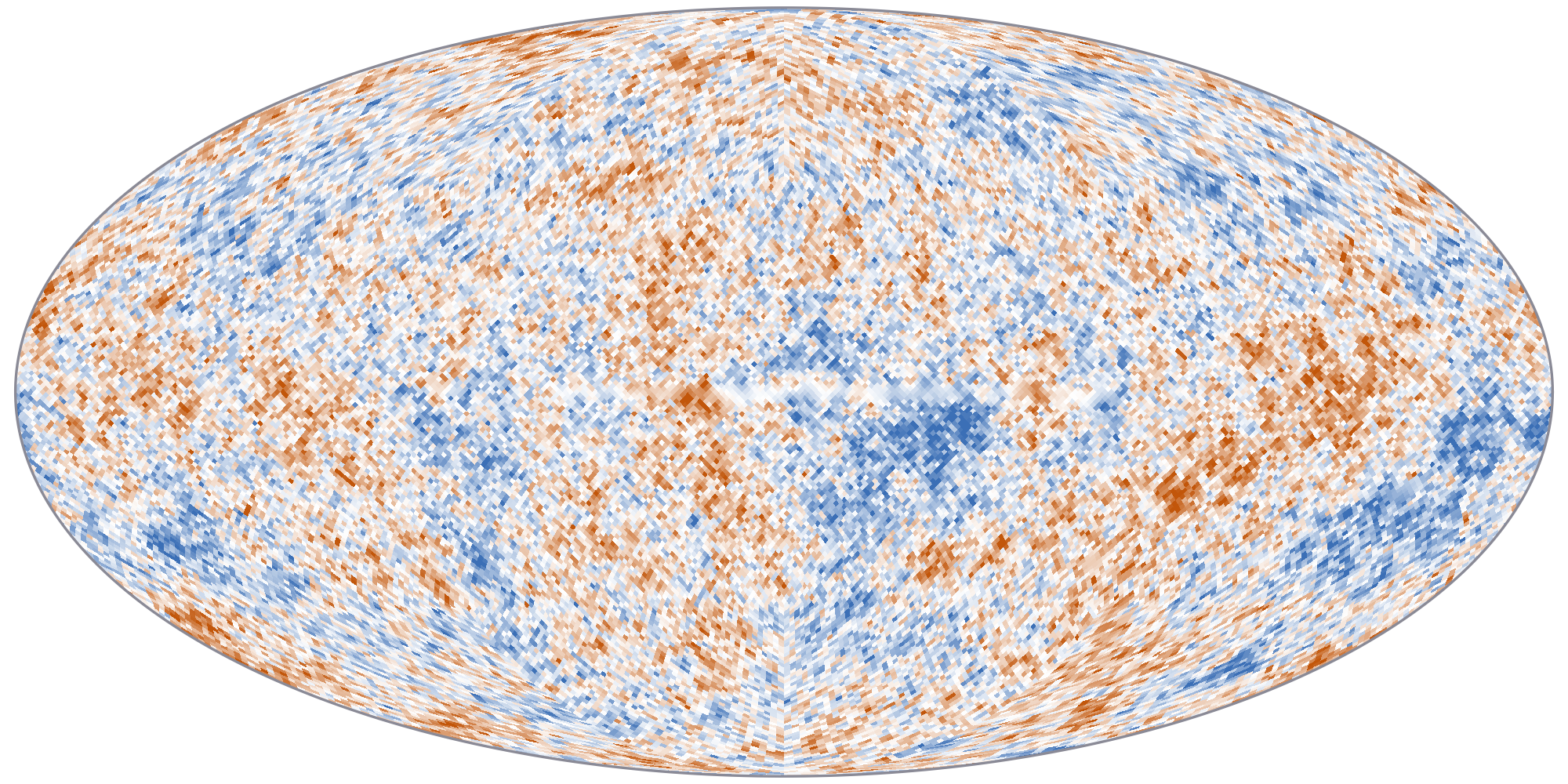
\(N_\mathrm{side}\) \(= 64\)
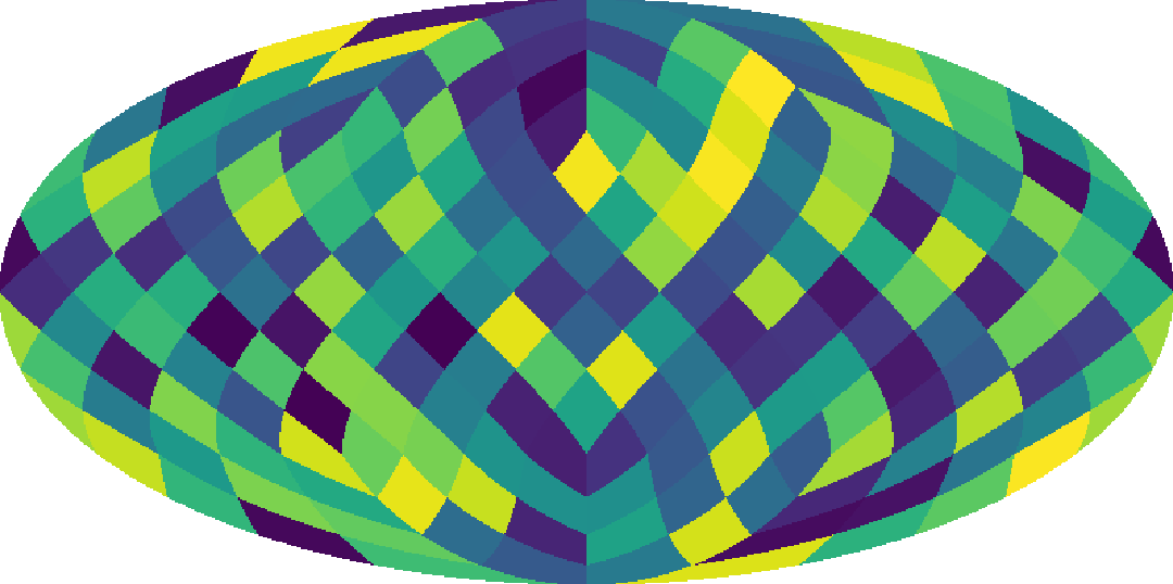
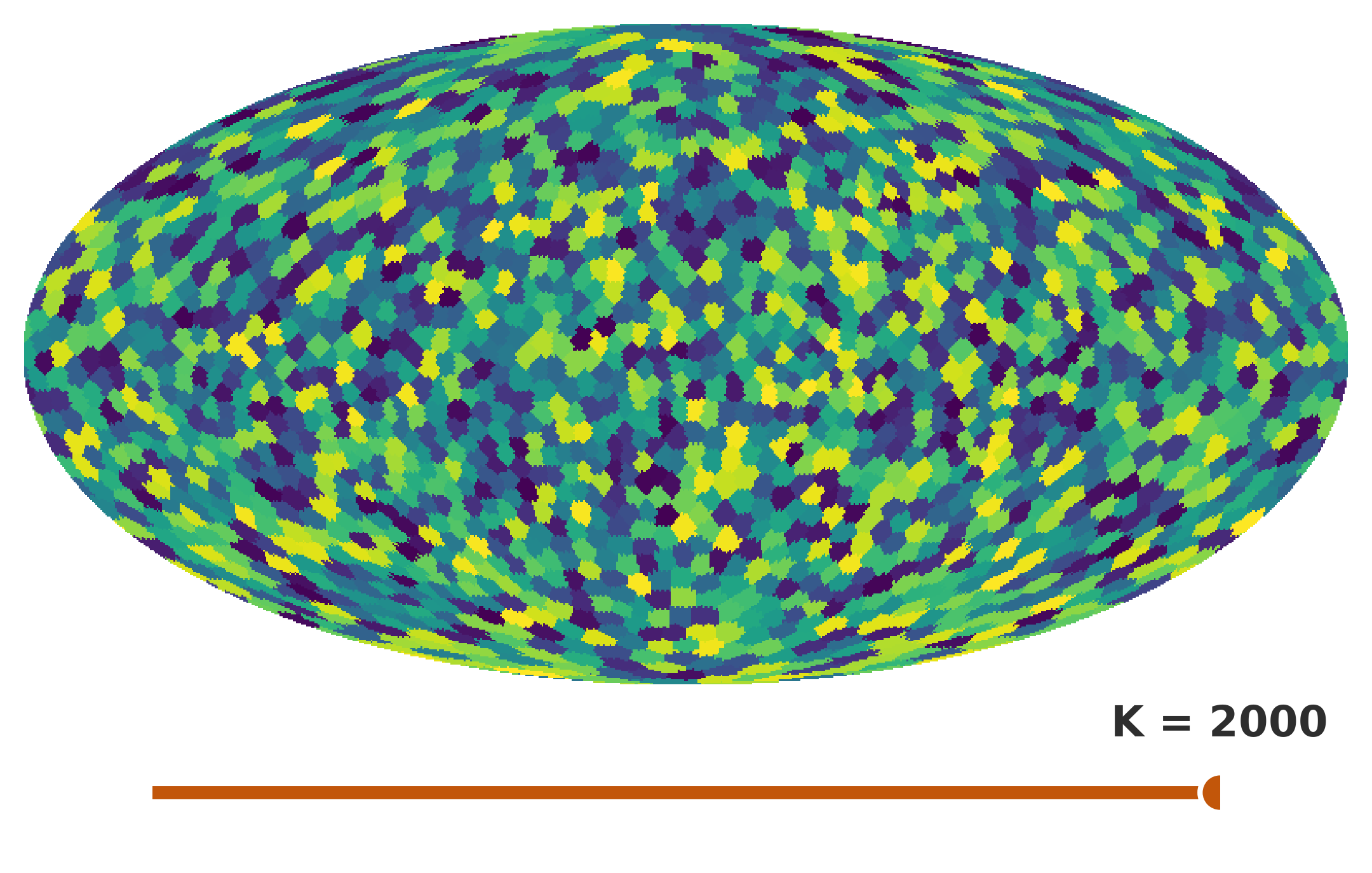
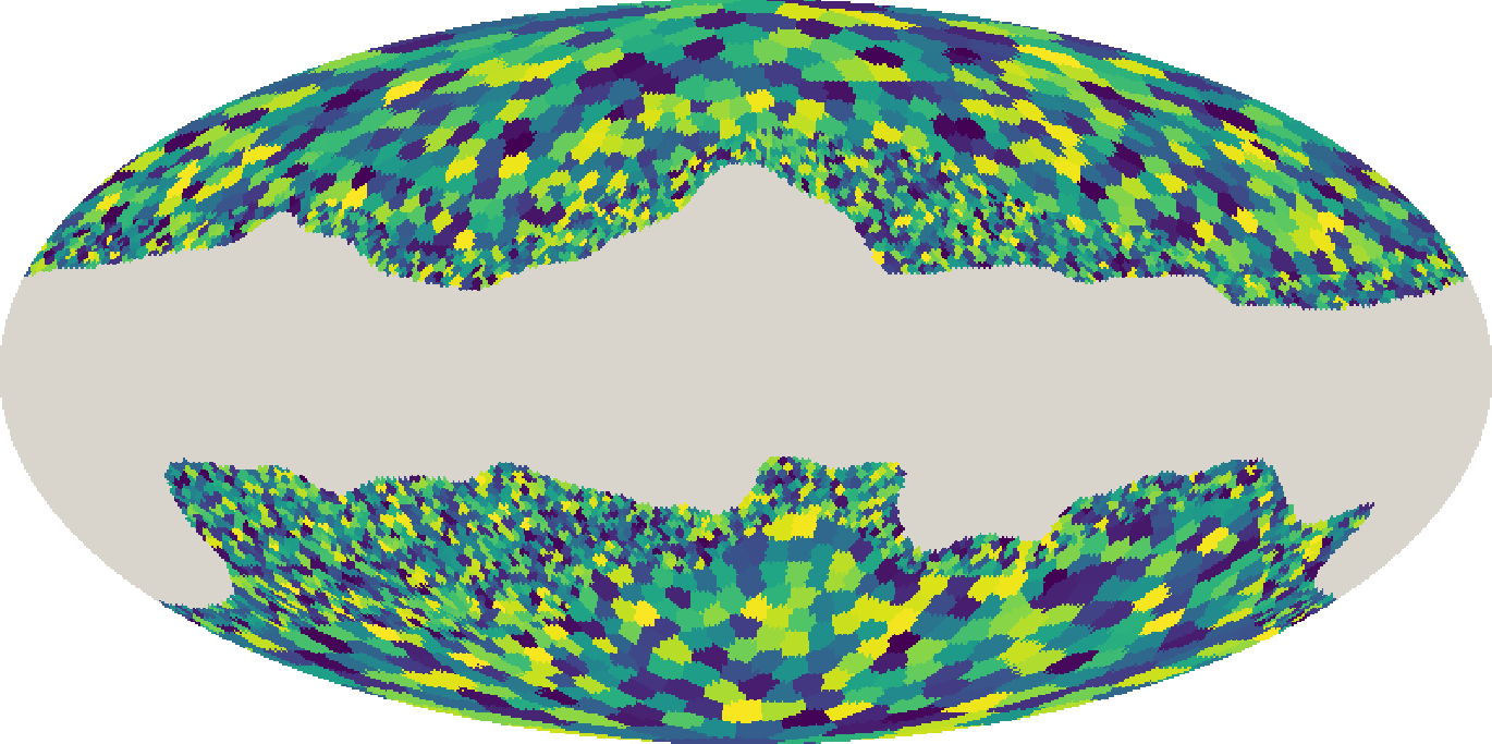
\(N_{\rm side} = 4\) · 192 patches
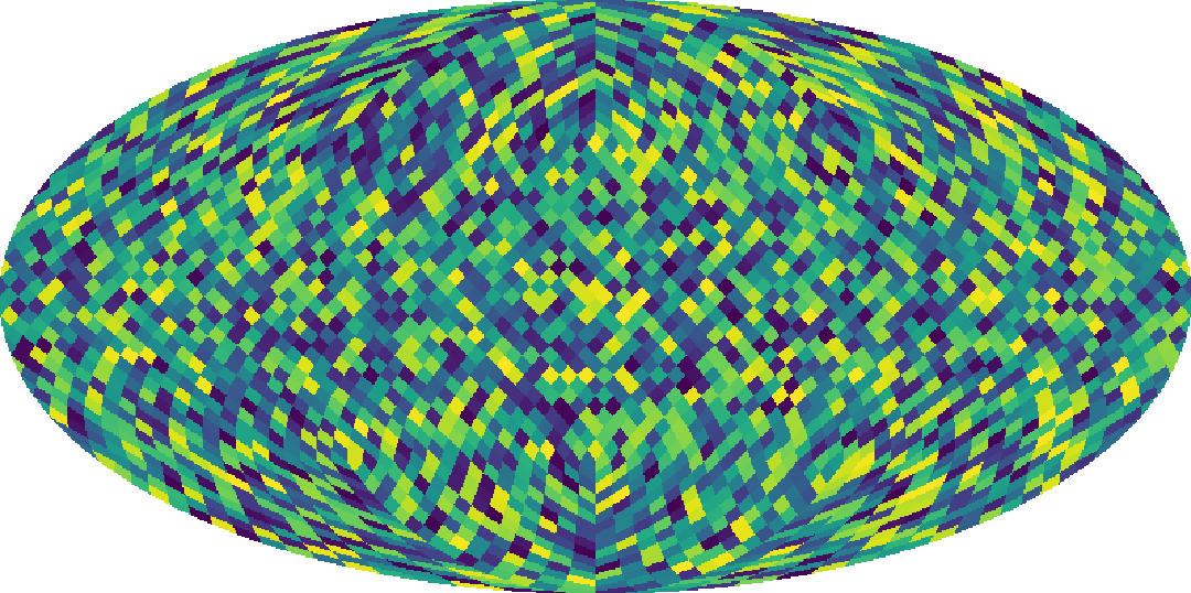
\(N_{\rm side} = 16\) · 3072 patches
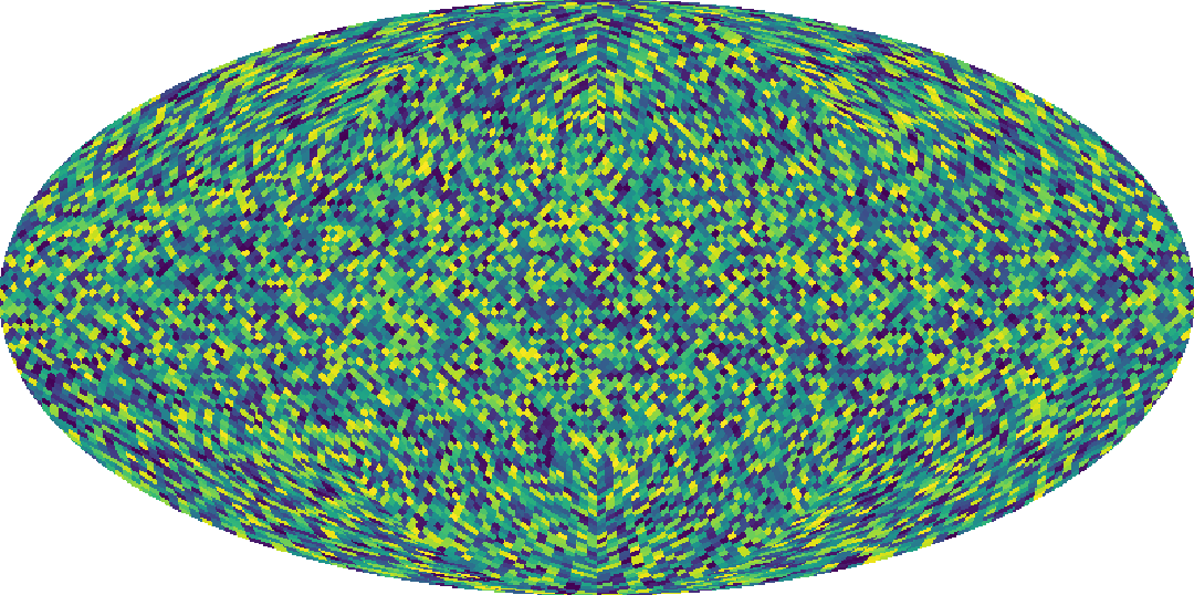
\(N_{\rm side} = 32\) · 12288 patches
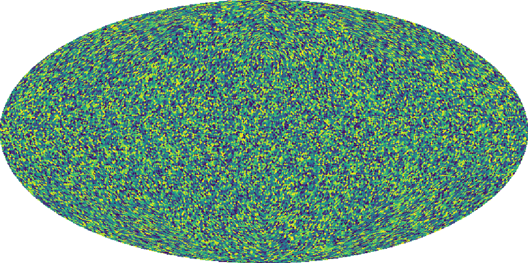
\(N_{\rm side} = 64\) · 49152 patches
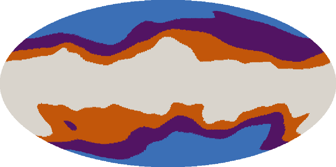
low · mid · high Galactic latitude, 20 % of the sky each
Planck Galactic masks: Planck Collaboration (2020), A&A 641, A4
\(N_{\rm side}\) per parameter in the LiteBIRD analysis
| low | mid | high | |
|---|---|---|---|
| \(\beta_d\) | 64 | 64 | 64 |
| \(T_d\) | 8 | 4 | 0 |
| \(\beta_s\) | 4 | 2 | 2 |
per Galactic region (0: one patch)
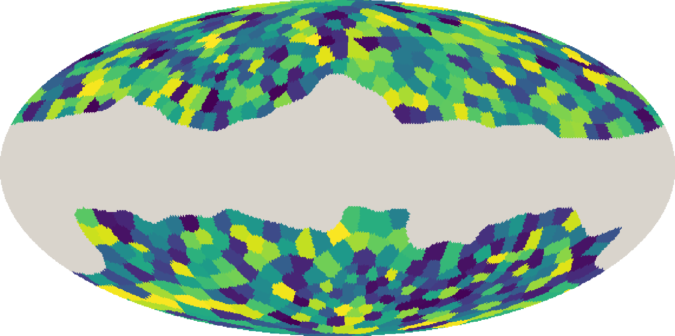
Example: the \(T_d\) partition
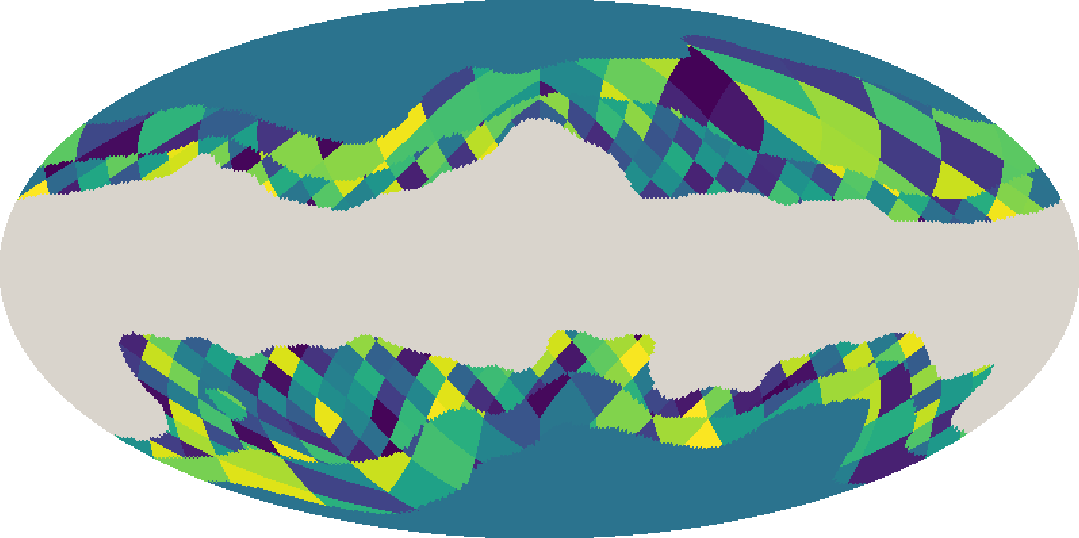
\(T_d\) at \(N_{\rm side}\) 8 / 4 / 0 · 344 patches


Obstacle for full-sky CMB surveys: LiteBIRD
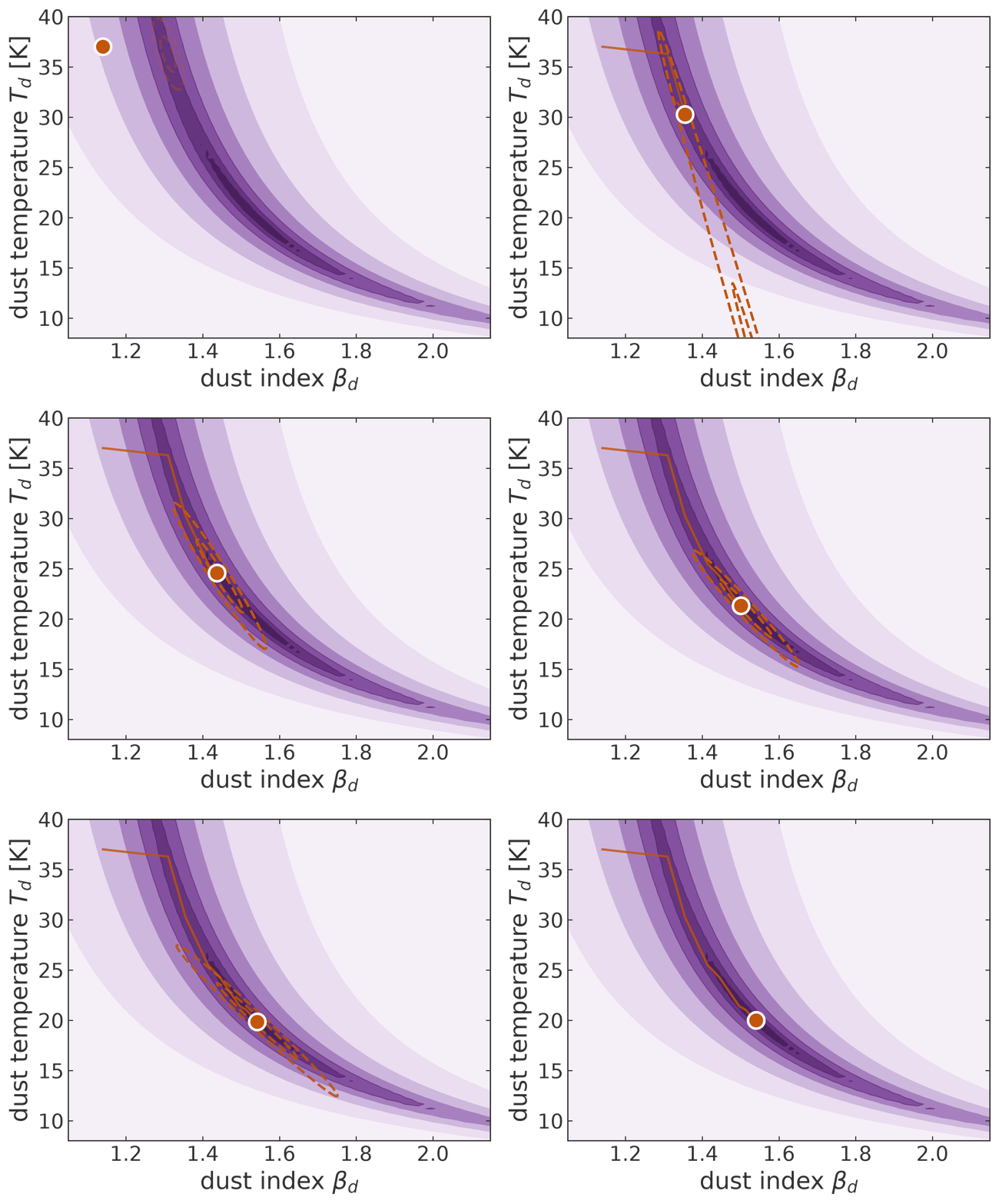
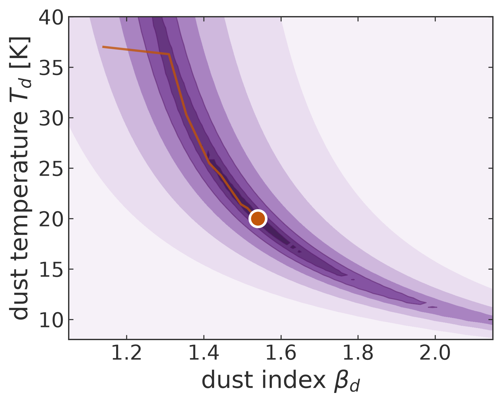
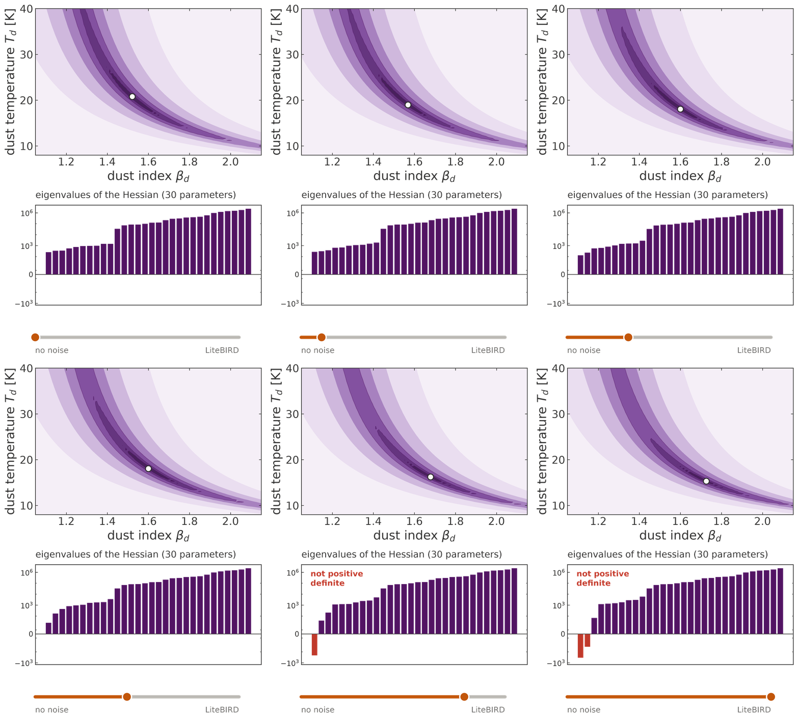
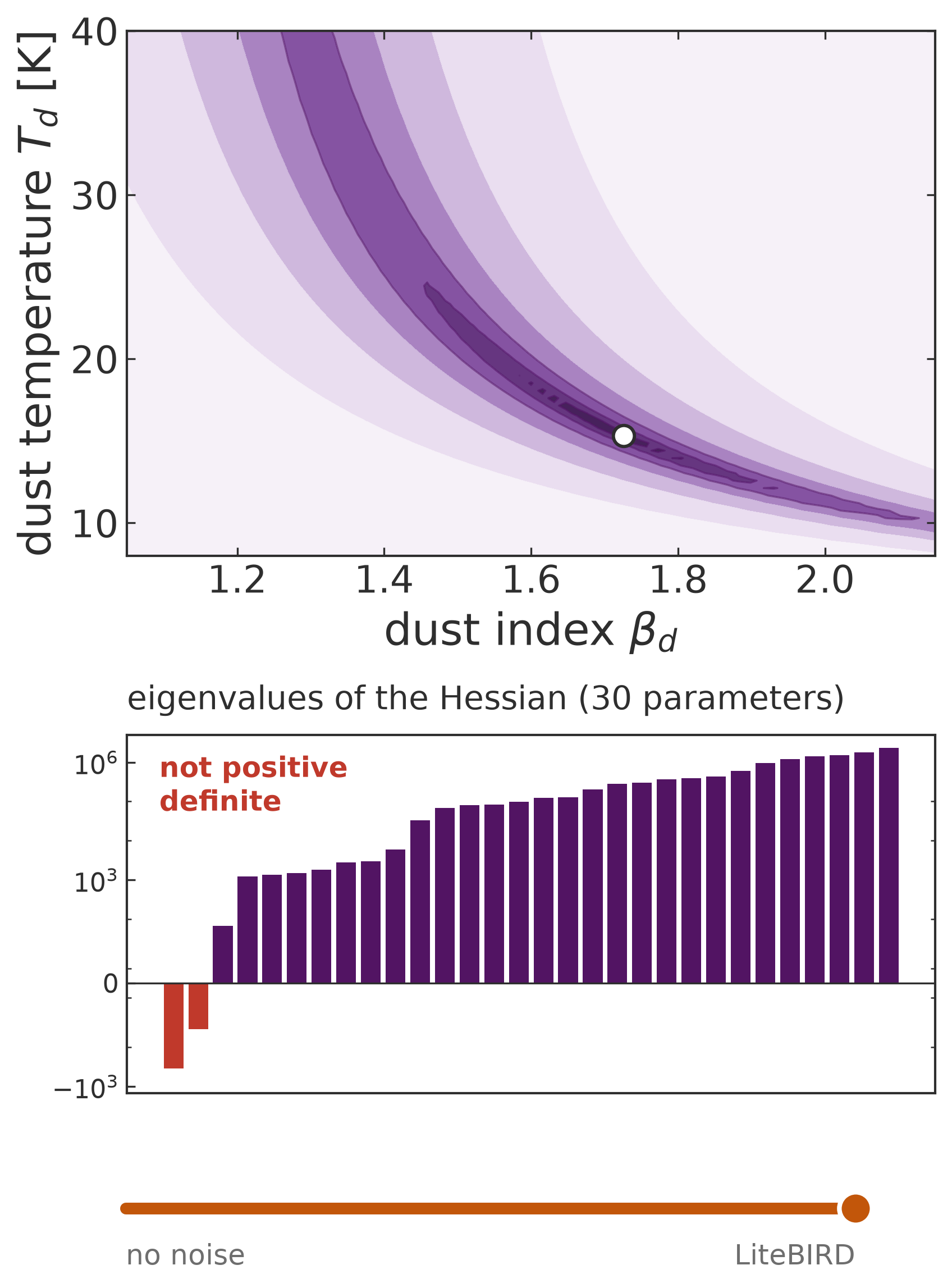
The Newton method
\[\boldsymbol\beta_{k+1} = \boldsymbol\beta_k - \mathbf{H}_k^{-1}\,\mathbf{g}_k\] \[\mathbf{g} = \nabla_{\boldsymbol\beta}\left(-\ln\mathcal{L}\right), \qquad \mathbf{H} = \nabla^2_{\boldsymbol\beta}\left(-\ln\mathcal{L}\right)\]
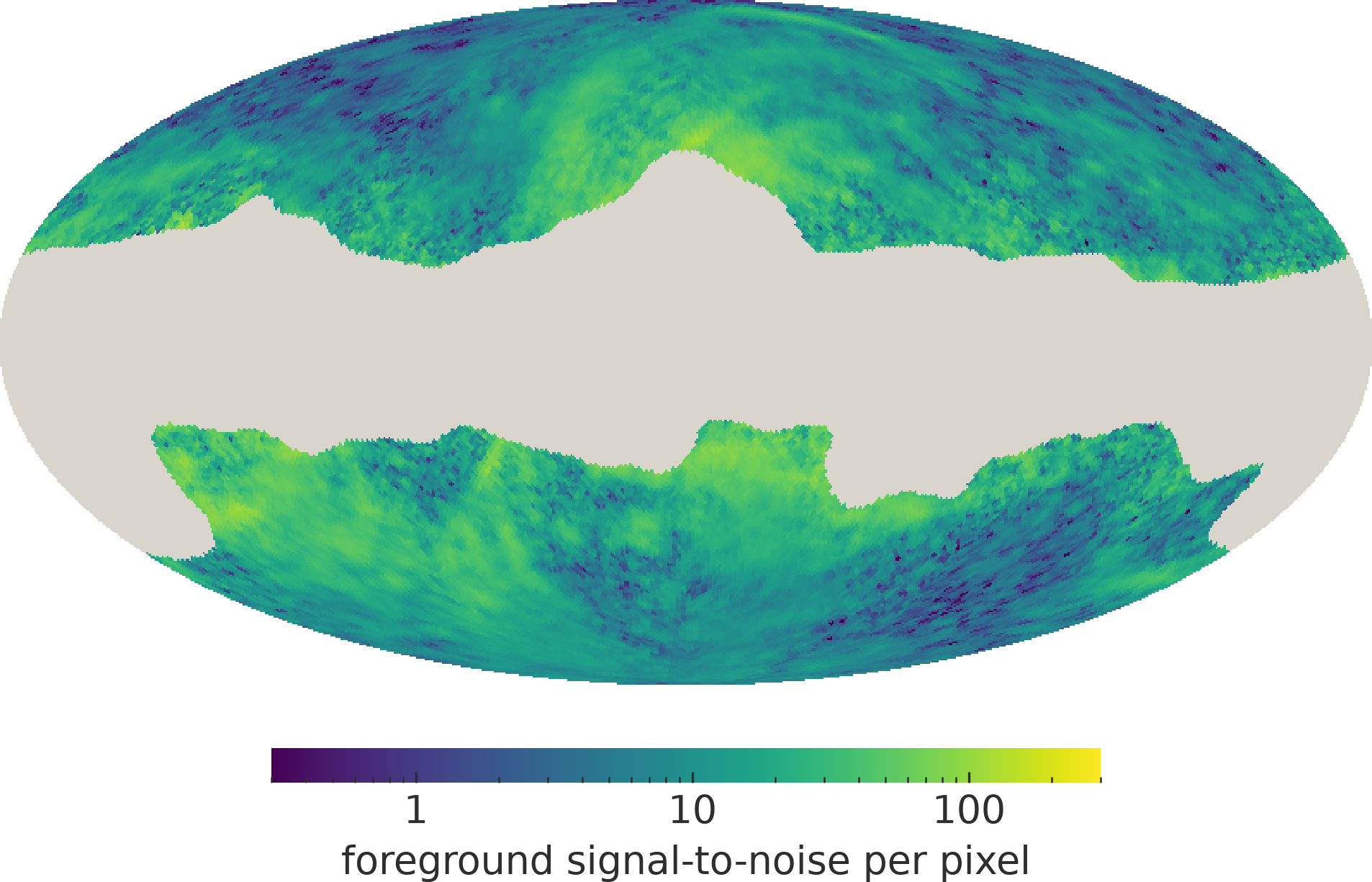
140 GHz, LiteBIRD depth

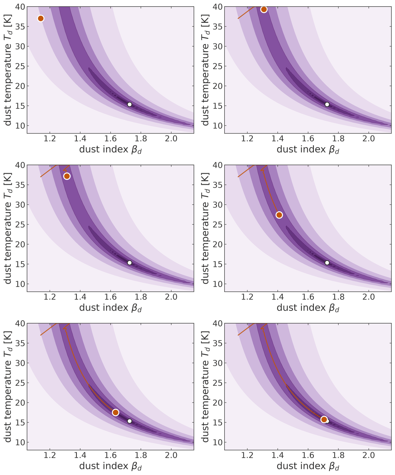
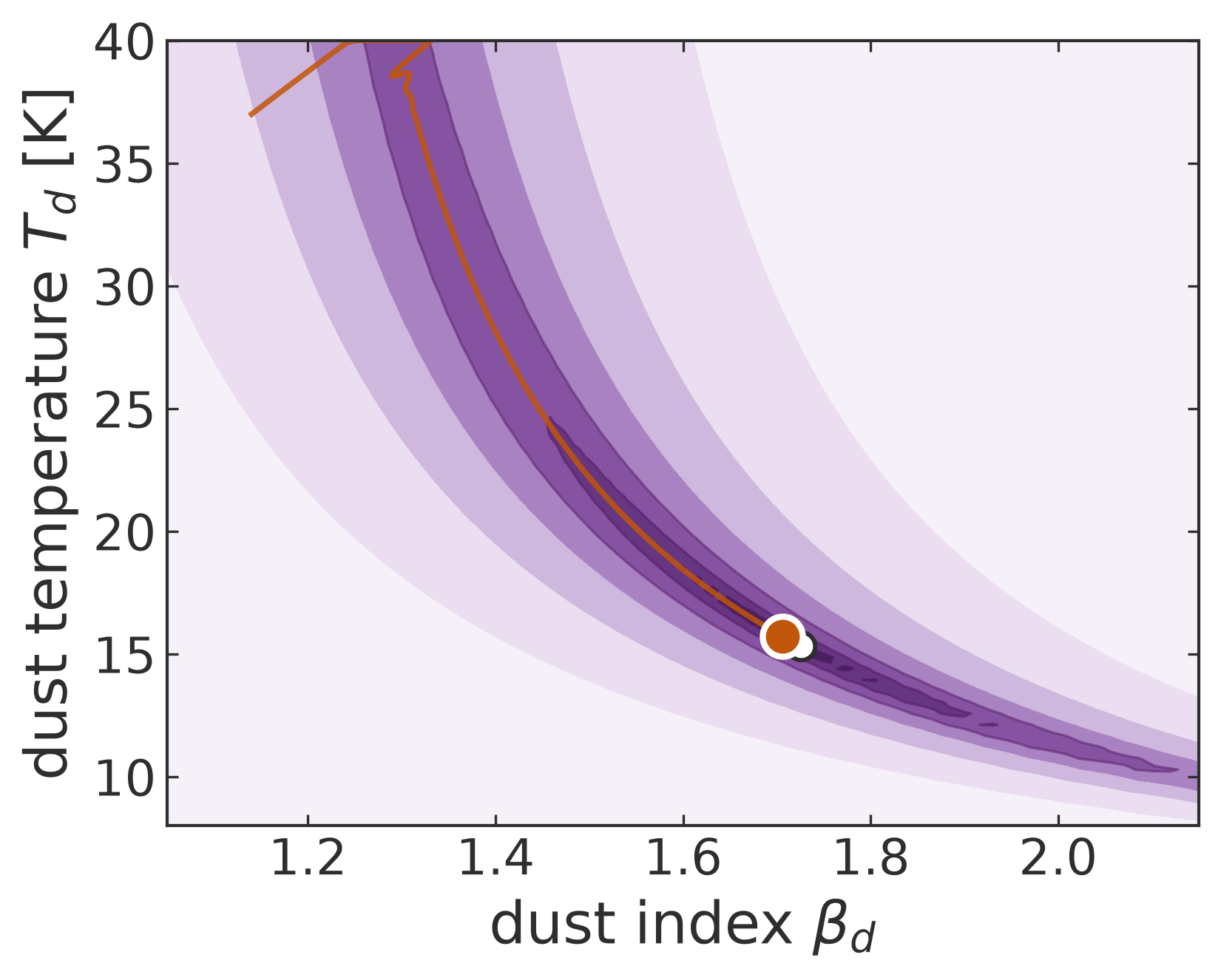
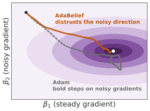
Adam is the standard optimiser of machine learning, built for very many parameters and very noisy gradients
\[\boldsymbol\beta_{t+1} = \boldsymbol\beta_t - \eta\,\frac{\hat m_t}{\sqrt{\hat v_t}+\epsilon}\]
\(m_t\), \(v_t\): running means of \(\mathbf{g}\) and \(\mathbf{g}^2\)
AdaBelief scales the step by the spread of the gradient instead
\[v_t \;\longrightarrow\; s_t:\ \text{running mean of }(\mathbf{g} - m_t)^2\]
A noisy direction gets a smaller step
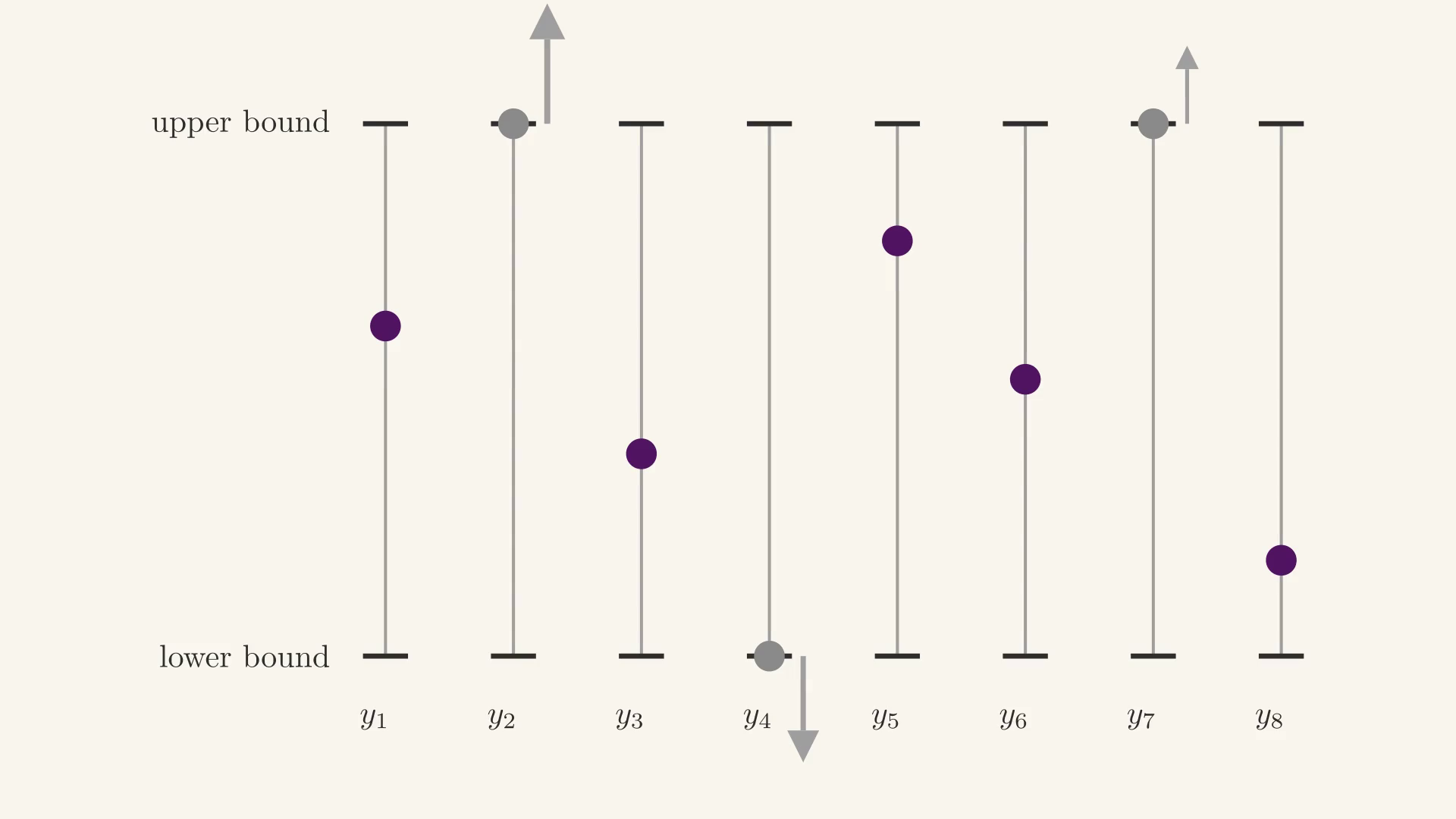
AdaTopK builds on AdaBelief for physical parameters, with a robust handling of parameter bounds
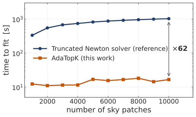
Scaling

Chanial, Biquard, Kabalan et al. (2026), FURAX, arXiv:2603.19600, submitted to JOSS
Kabalan et al. (2026), arXiv:2604.08463, submitted to RASTI
Jean Zay, IDRIS
NVIDIA H100 GPUs
We do this for each region
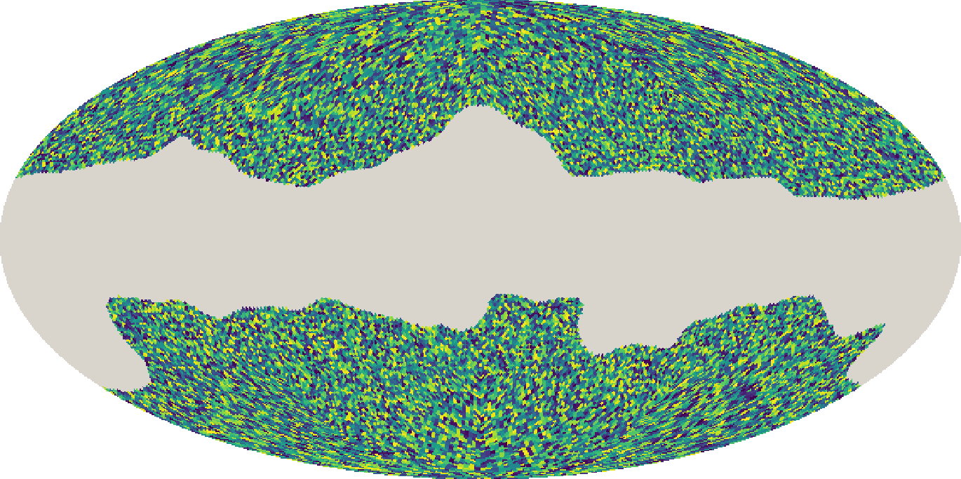
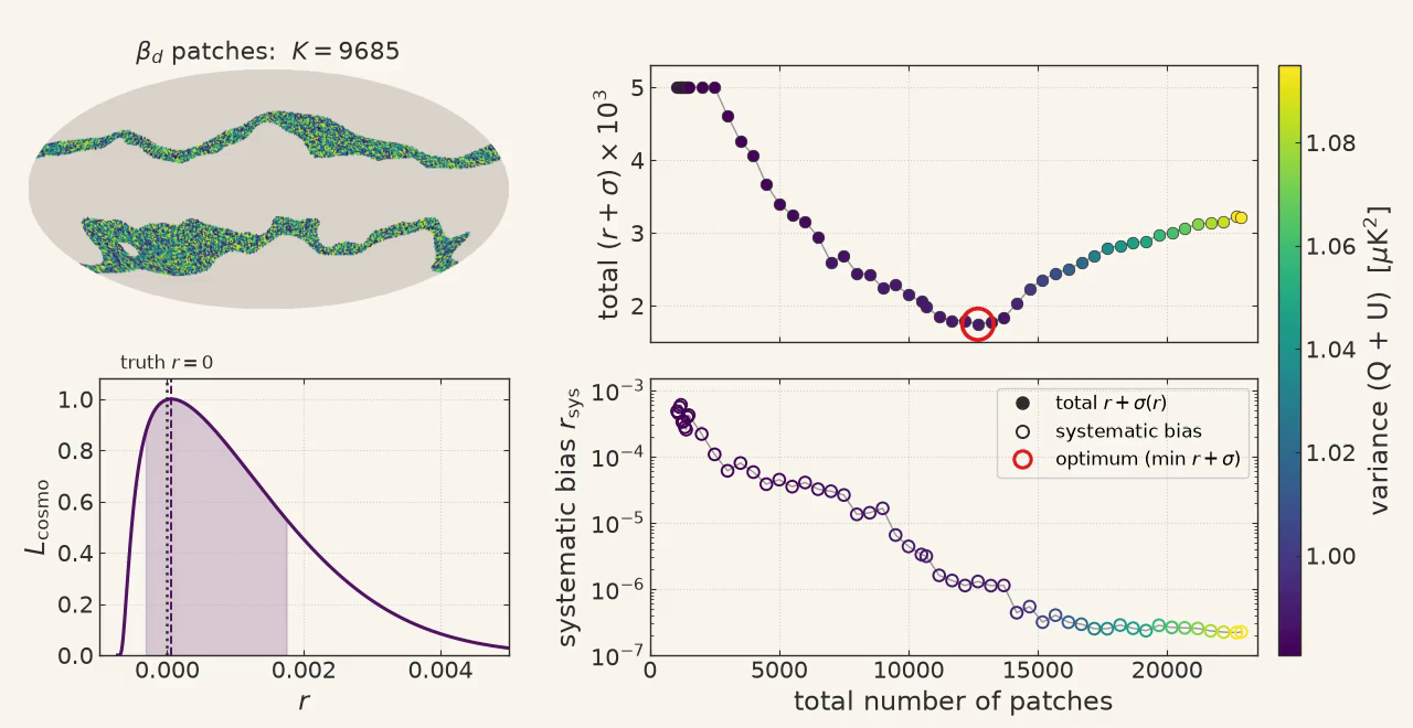
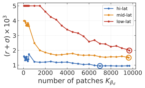
\(\beta_d\) patches
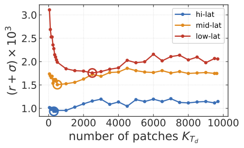
\(T_d\) patches
\(\beta_s\) patches
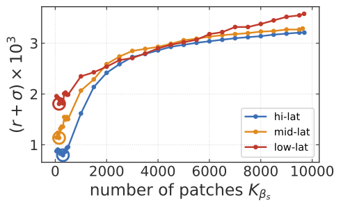
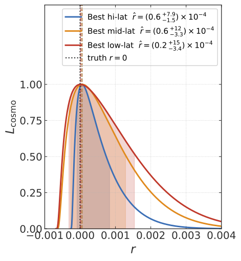
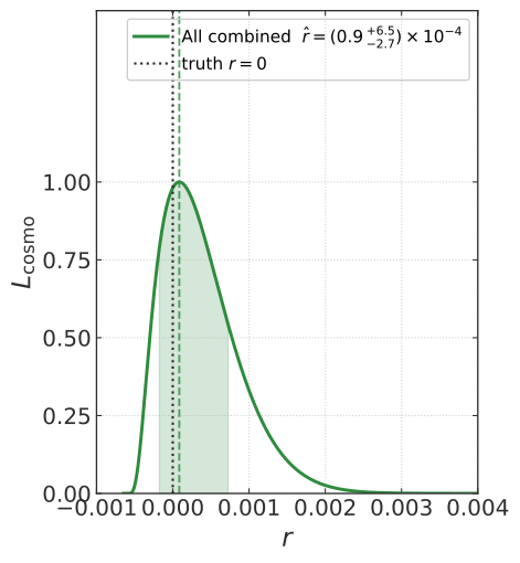
Run details
Over 10 000 component separation runs on 64 NVIDIA H100 GPUs
Finishing in 10 hours
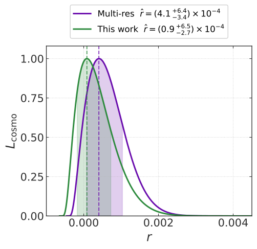
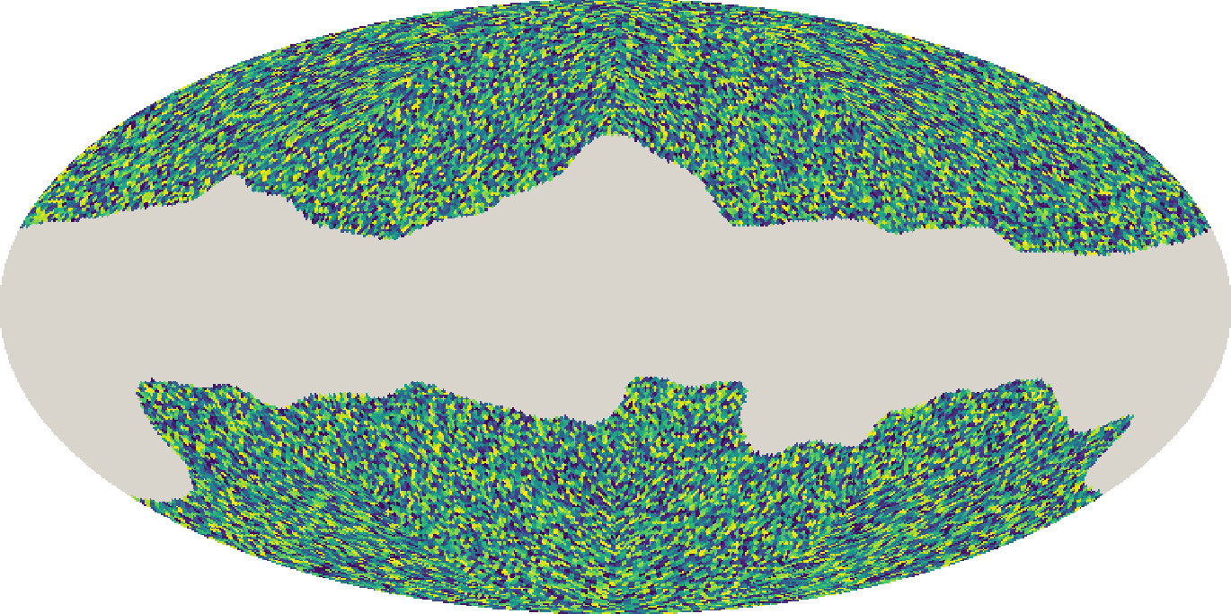
\(\beta_d\)
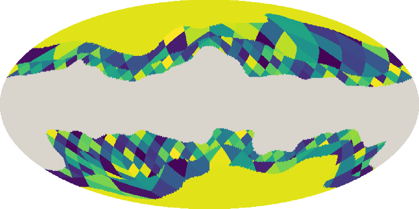
\(T_d\)
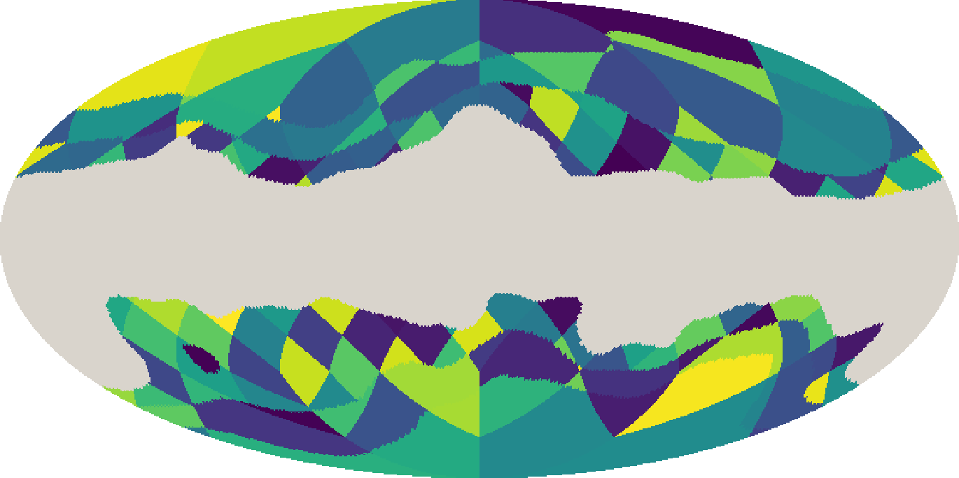
\(\beta_s\)
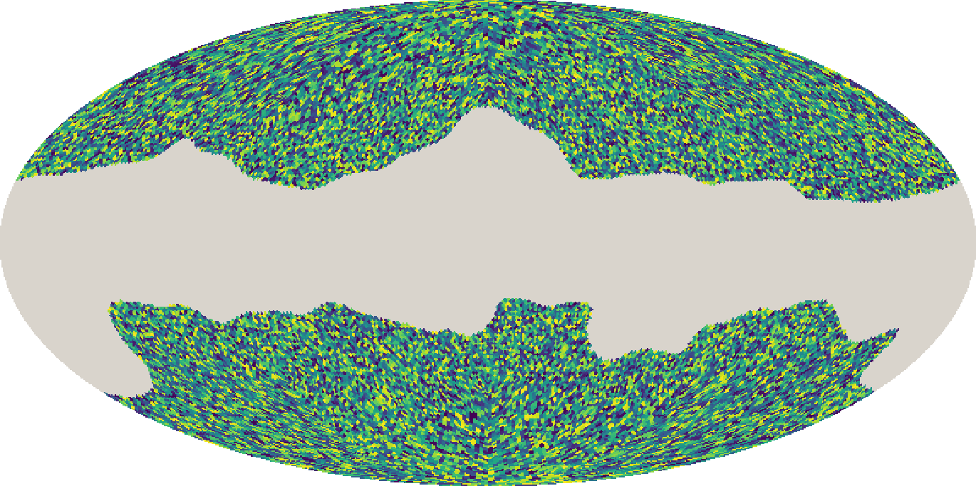
\(\beta_d\)
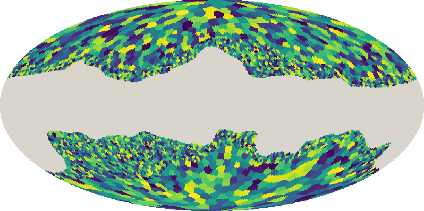
\(T_d\)
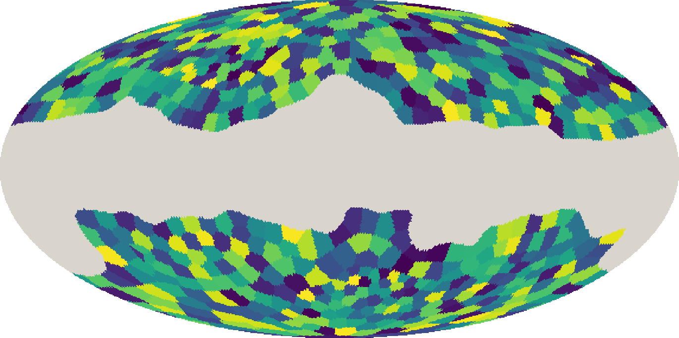
\(\beta_s\)
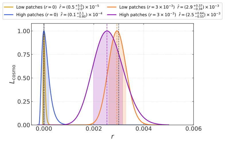
30 % lower 68 % upper limit on \(r\), with the same instrument, sky and noise: only the partition changes
Kabalan et al. (2026), JAX-accelerated parametric CMB component separation, submitted to RASTI
Now part of the Megatop pipeline for the Simons Observatory
Perspectives


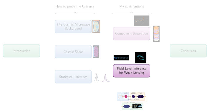
Kabalan et al. (2026) · submitted to RASTI
Kabalan et al. (2026b) · accepted to JOSS
Kabalan et al. (2026c) · in prep. for JCAP

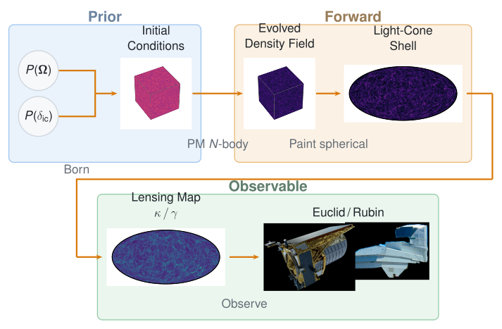
From a cosmology and an initial density field to convergence and shear on the curved sky
A fast and differentiable gravity solver that can simulate Stage IV survey volumes
Each particle moves from its initial grid position \(\mathbf{q}\)
\[\mathbf{x}(\mathbf{q}, a) = \mathbf{q} + D_1(a)\,\mathbf{\Psi}^{(1)}(\mathbf{q}) + D_2(a)\,\mathbf{\Psi}^{(2)}(\mathbf{q}) + \dots\] \[\nabla \cdot \mathbf{\Psi}^{(1)} = -\delta_\mathrm{ini}\]
First order: the Zel’dovich approximation.
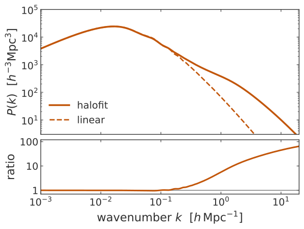
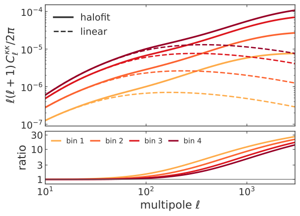
Matter power spectrum at \(z=0\), linear theory against halofit

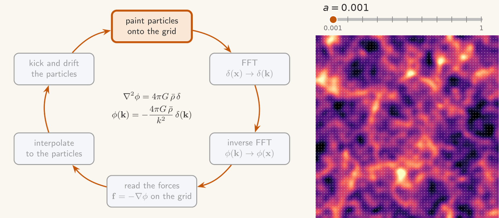
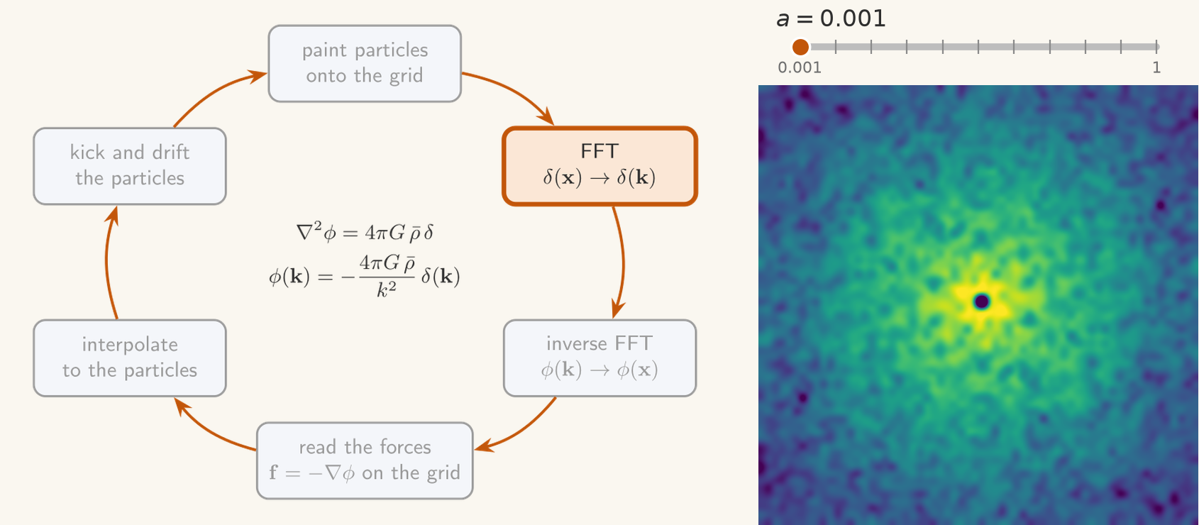
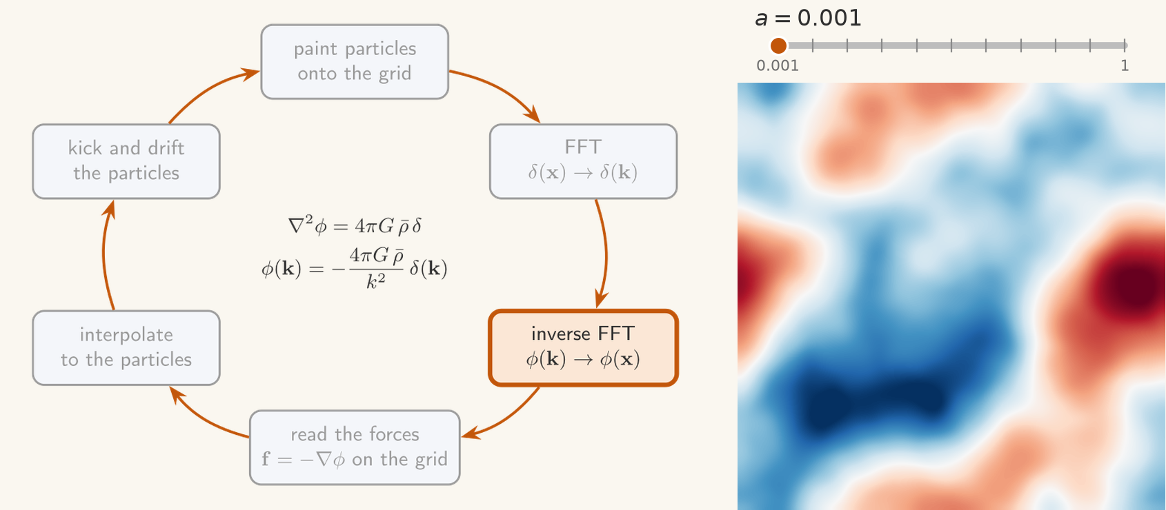
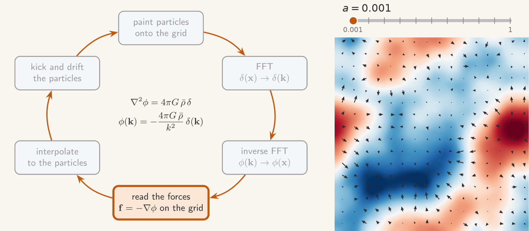
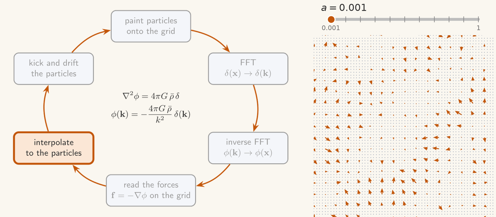
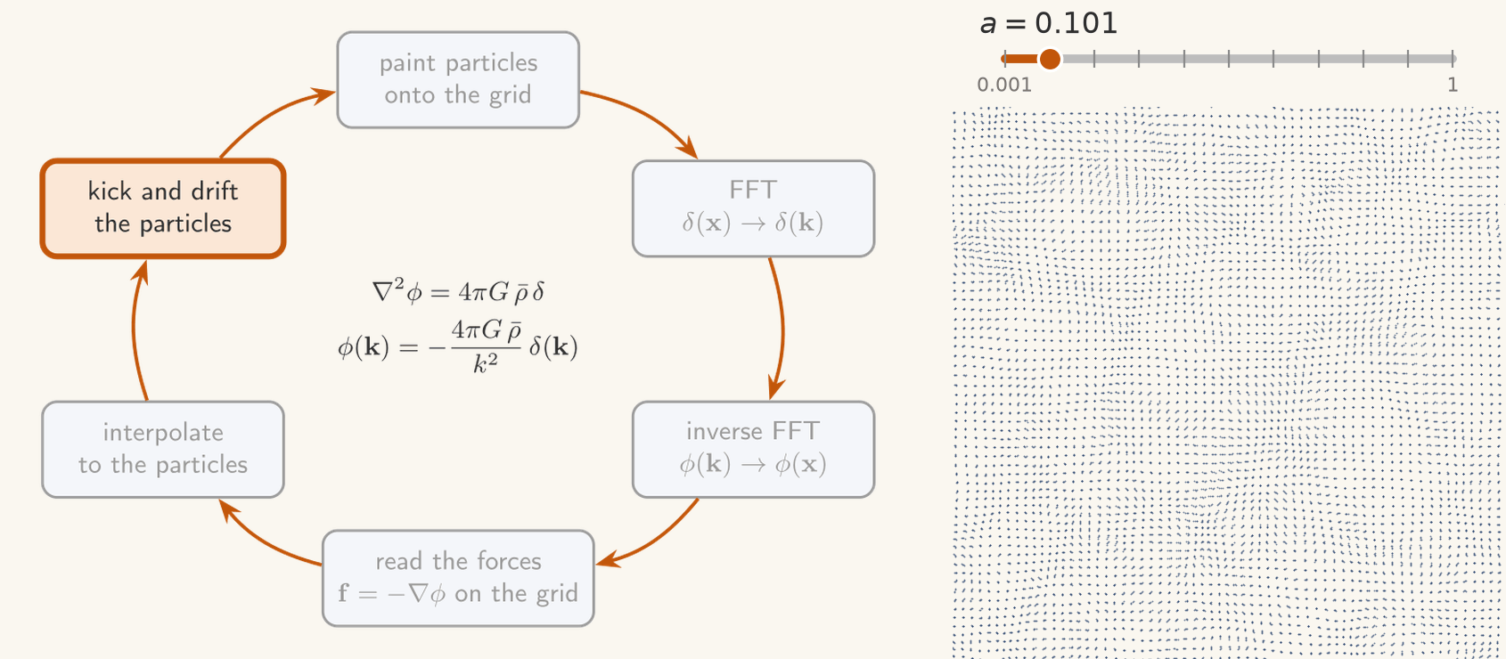
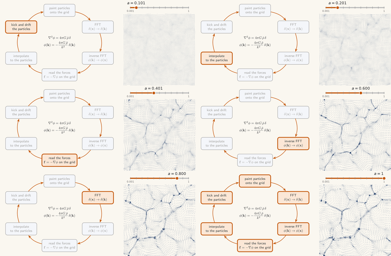
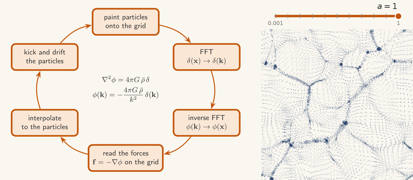
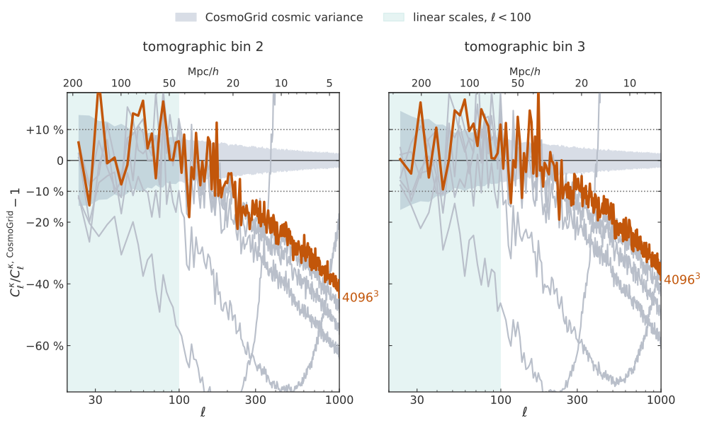
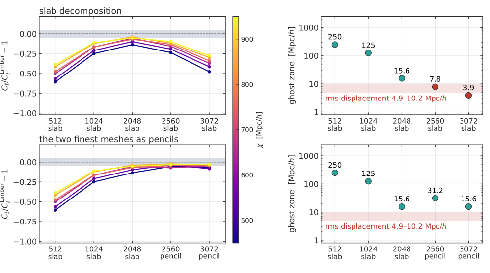
Gravity through FFTs on a mesh: fast, differentiable, and limited by the mesh resolution
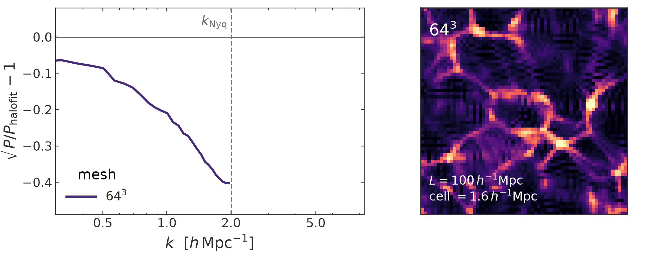
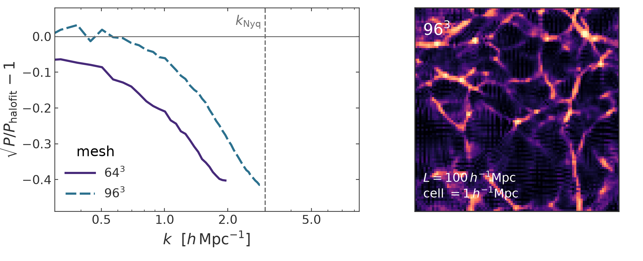
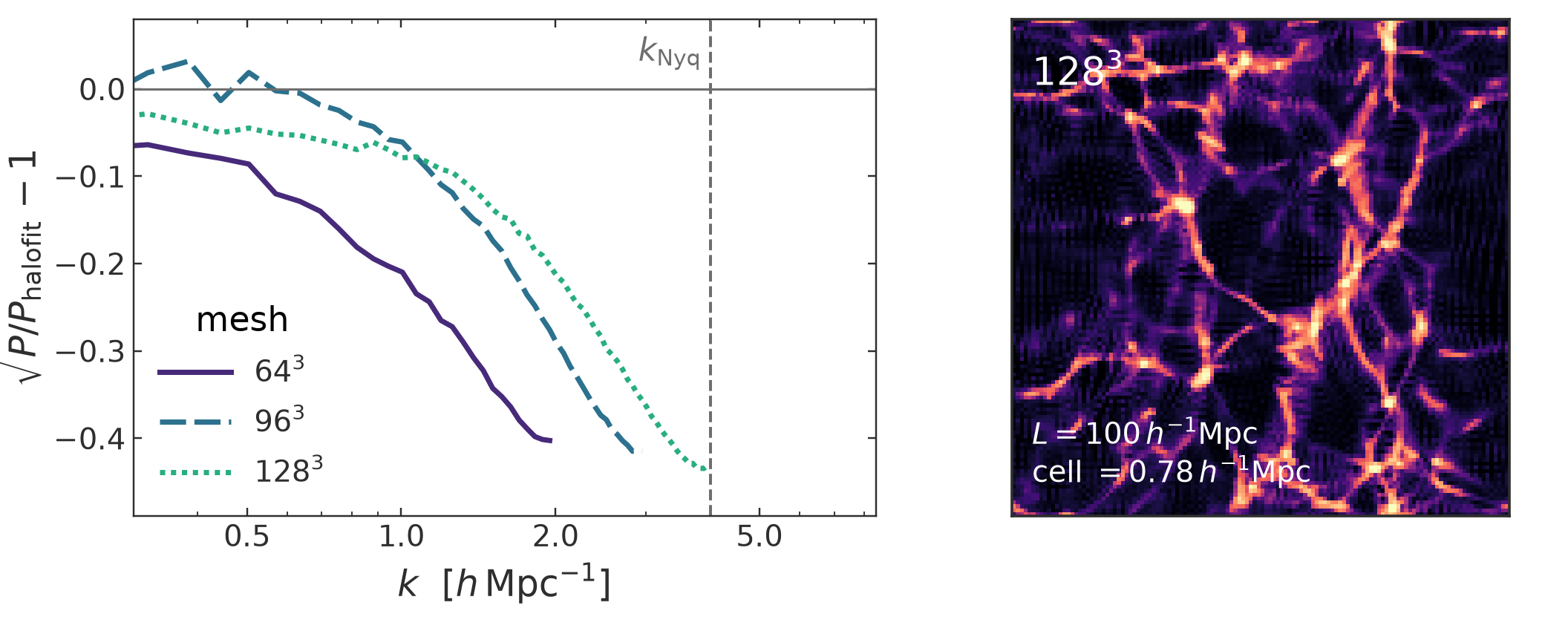
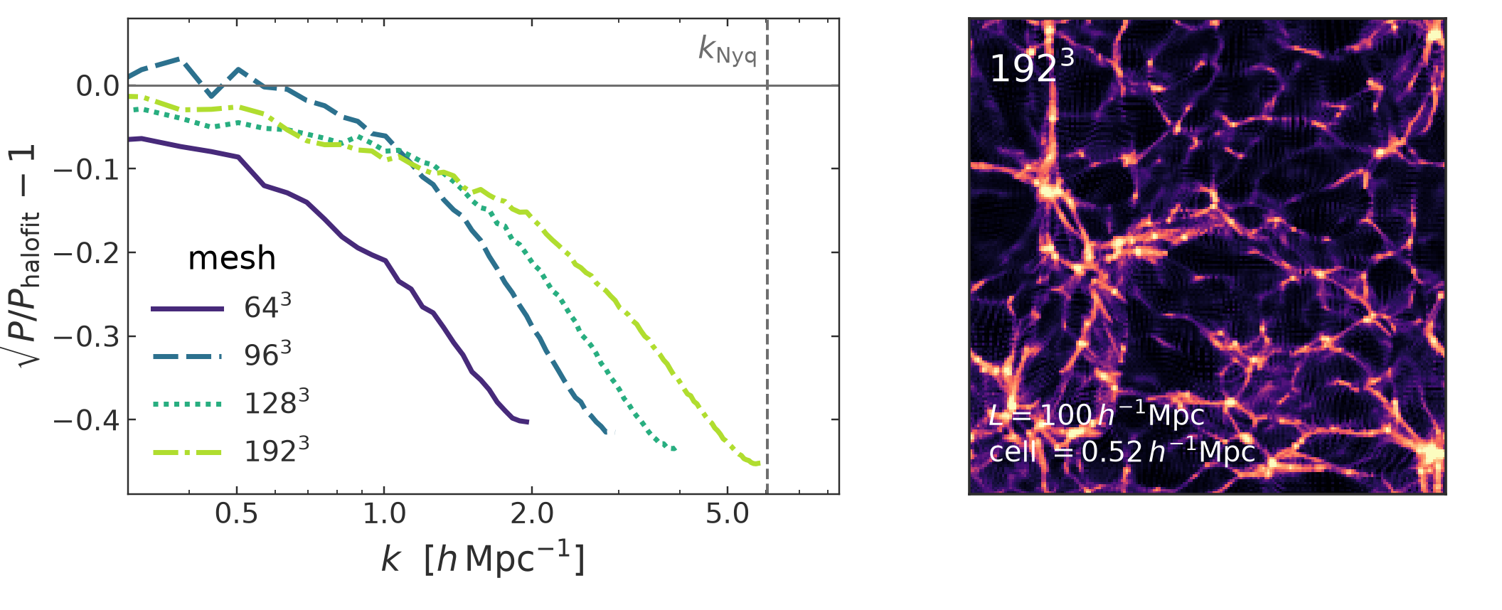
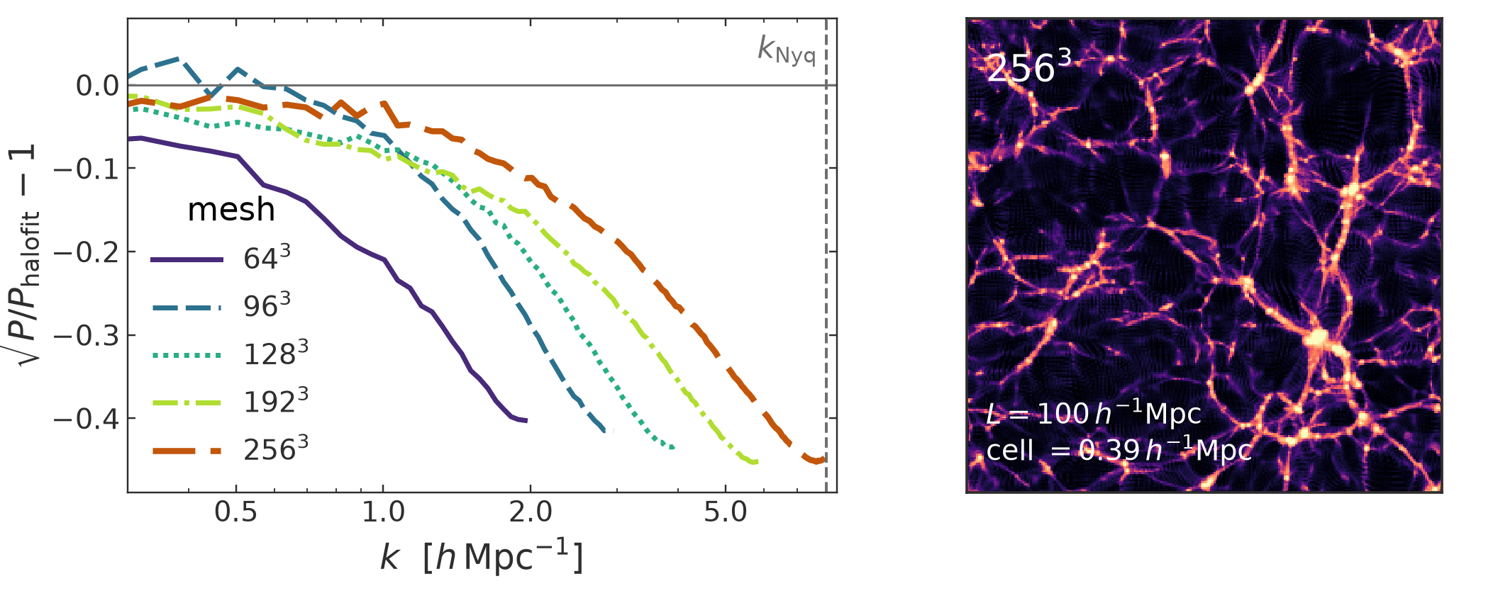

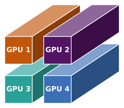
Kabalan et al. (2026b), jaxDecomp: JAX library for 3D domain decomposition and parallel FFTs, accepted to JOSS
Simulation-based inference on real survey data
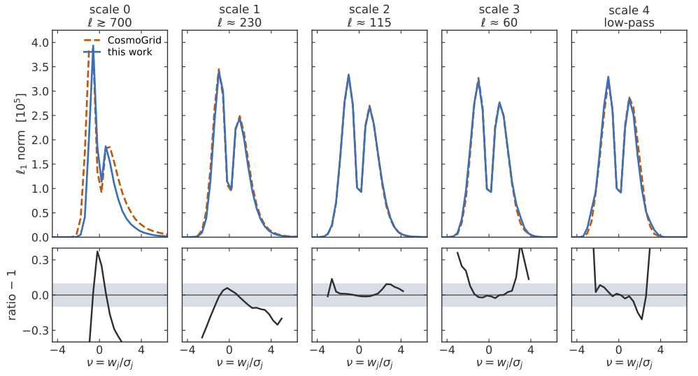
Applied on DES Y3, Jeffrey et al. (2024): SBI on real data using Gower Street Similations and validated on CosmoGridV1.
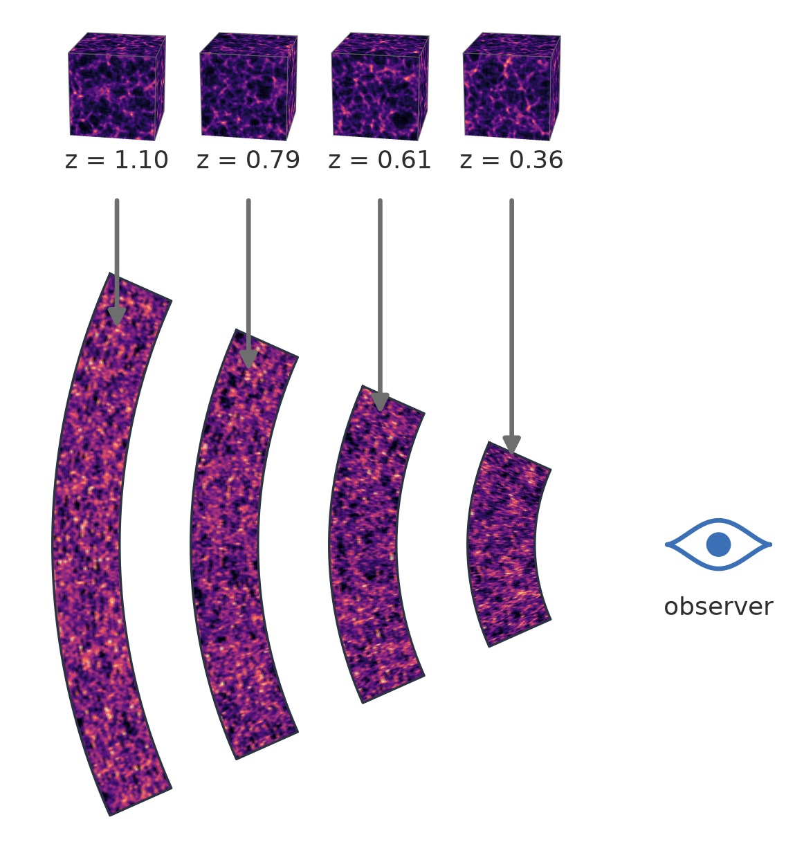
Born approximation: straight lines of sight
\[\kappa(\hat{\mathbf n};\chi_s) = \frac{3}{2}\,\Omega_m\Big(\frac{H_0}{c}\Big)^2 \sum_j W_j(\chi_s)\,\delta_j(\hat{\mathbf n})\]
\[W_j(\chi_s) = \int_{\mathrm{shell}\ j} \mathrm{d}\chi\;\chi\,(1+z)\Big(1-\frac{\chi}{\chi_s}\Big)\]
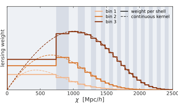
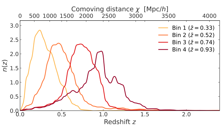
\[\kappa_i(\hat{\mathbf n}) = \int \mathrm{d}z\; n_i(z)\,\kappa\big(\hat{\mathbf n};\chi_s(z)\big)\]
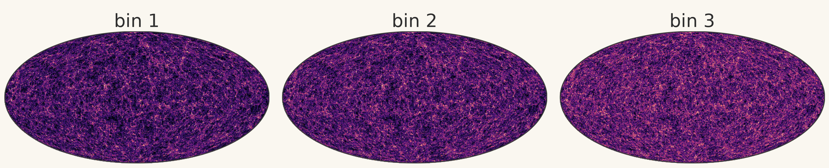
The Born approximation computes the convergence along undeflected light rays
Post-Born ray tracing computes deflection angle, but its correction to the convergence power spectrum is below the arcminute scale.
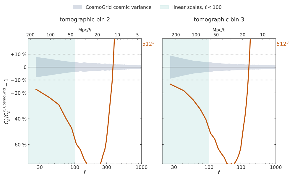
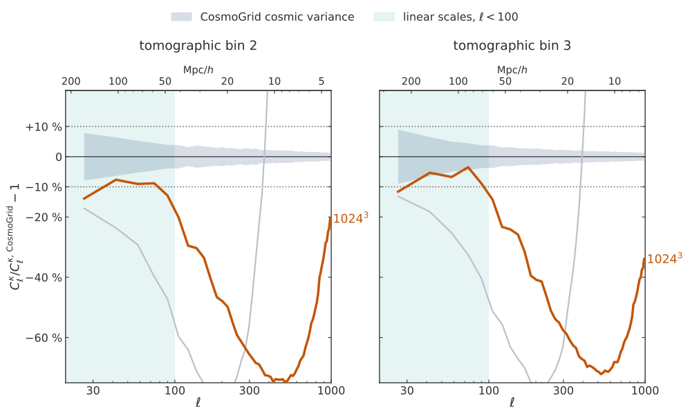
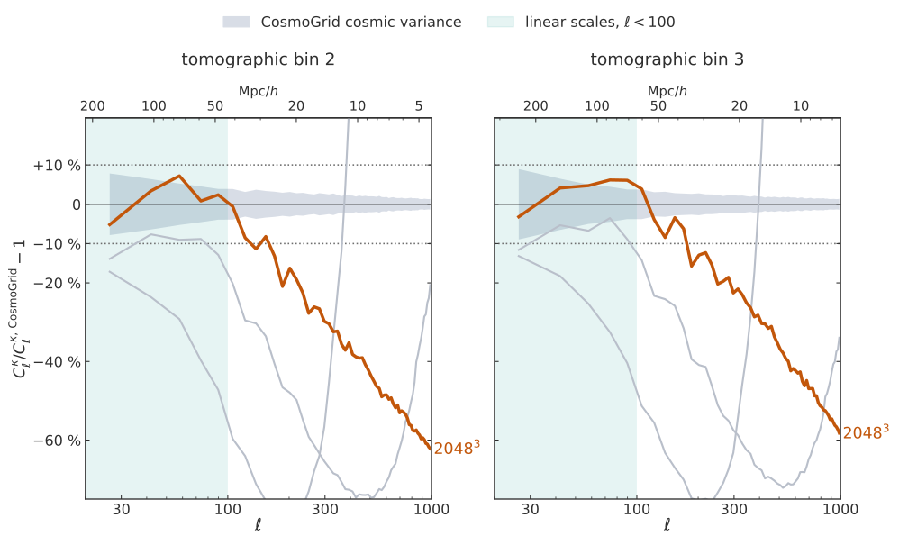
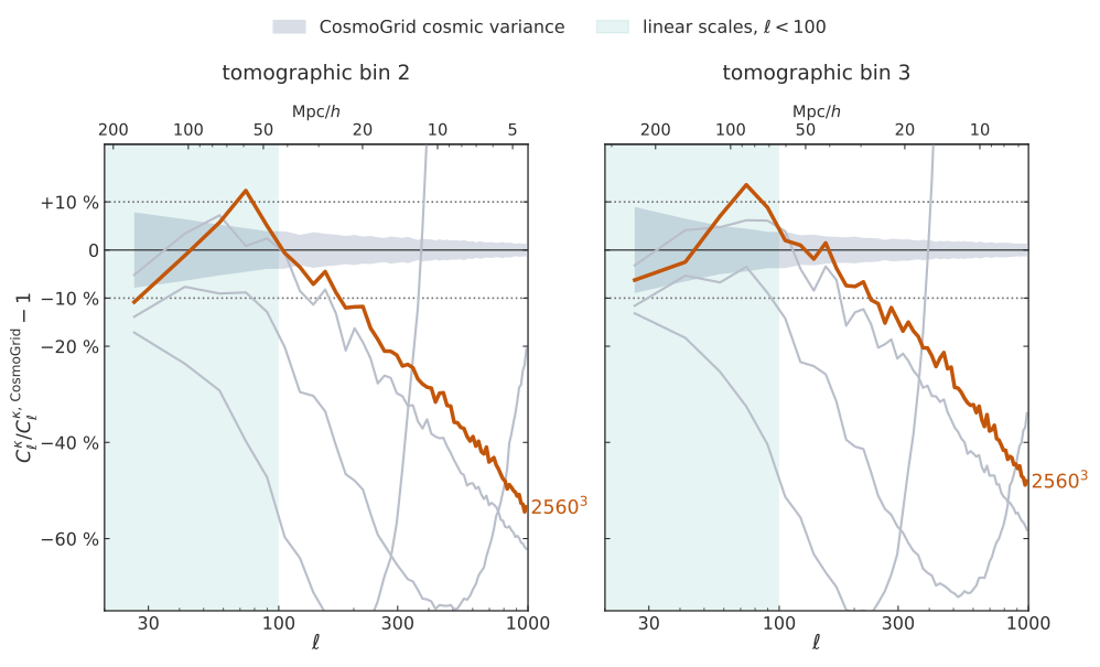
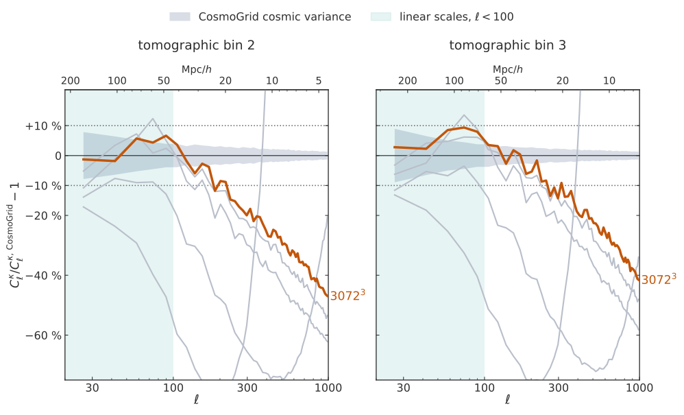
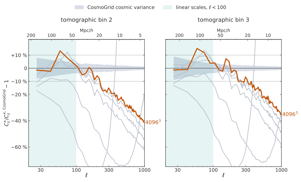
Kabalan et al. (2026c), in prep. for JCAP
Preliminary
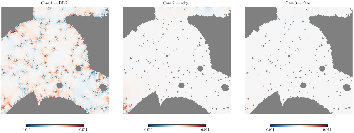
DES Y3 noise, \(1200^3\) mesh, 2LPT
\(N_\mathrm{side} = 1024\), painted at \(512\), \(\ell \le 700\)
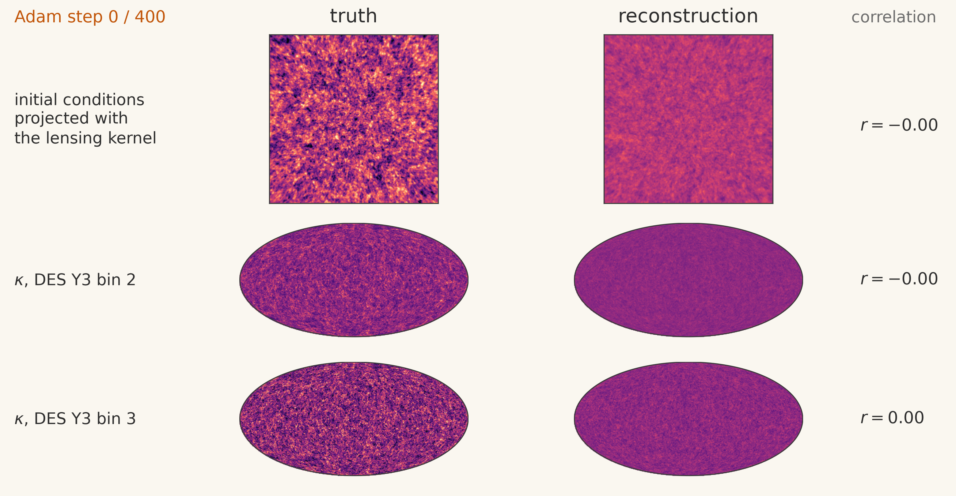
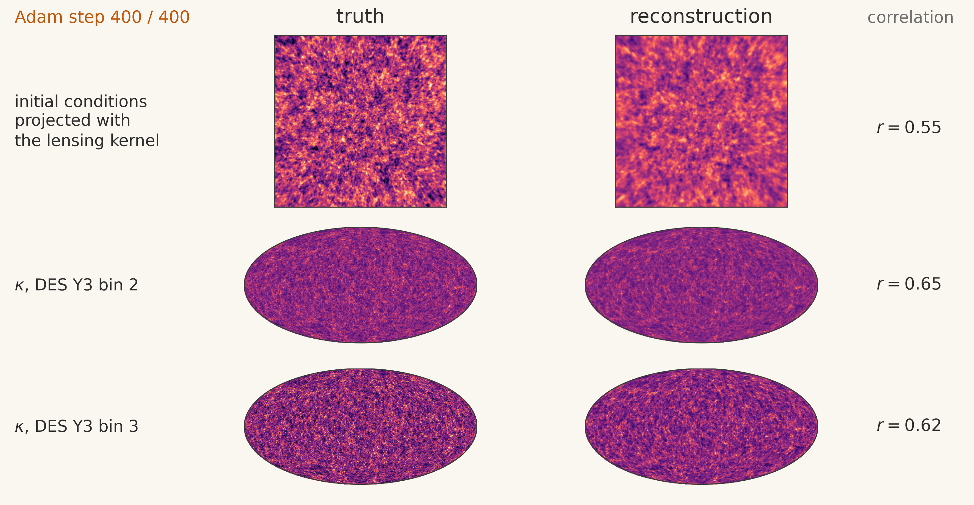
Kabalan et al. (2026b), jaxDecomp, accepted to JOSS · Kabalan et al. (2026c), in prep. for JCAP
Perspectives
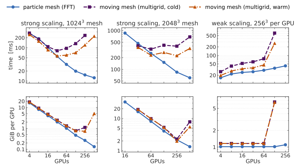
Moving-mesh particle mesh
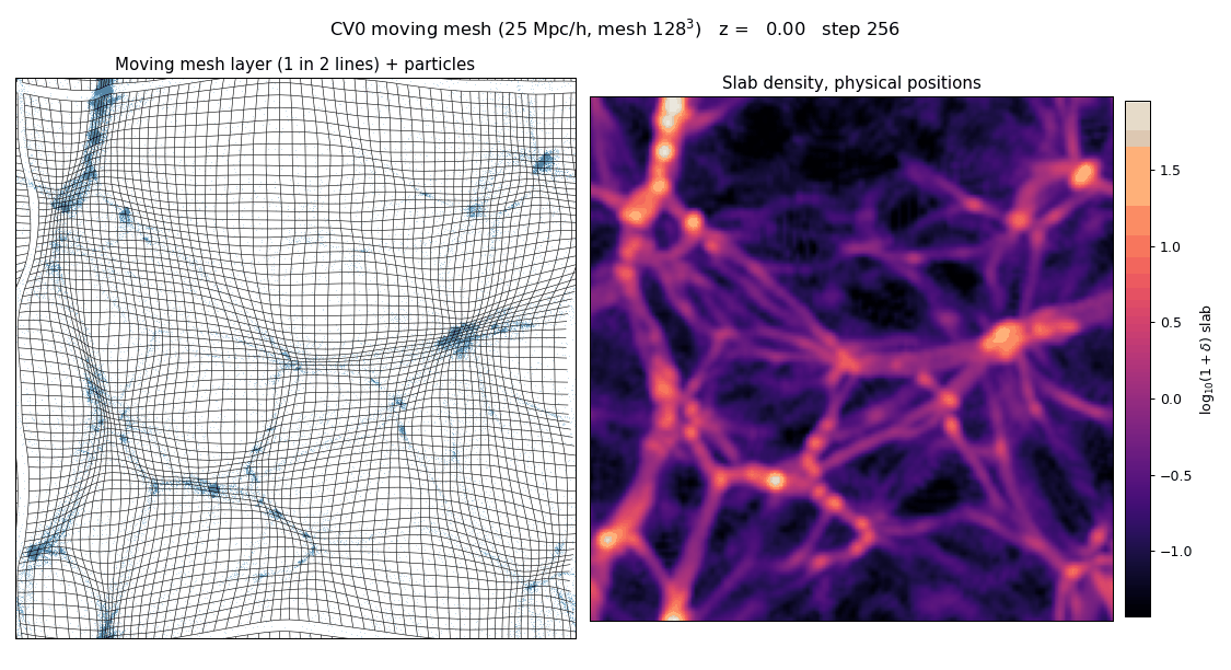
Moving mesh: B. Horowitz (2026), arXiv:2607.10983
Kabalan et al. (2026) · submitted to RASTI
Kabalan et al. (2026b) · accepted to JOSS
Kabalan et al. (2026c) · in prep. for JCAP
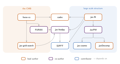
Reproducible software for research
Where it is used
furax-cs → the Megatop pipeline for the Simons Observatory; LiteBIRD component separation next
jax-healpy → used within the DESI collaboration
jaxDecomp → beyond cosmology: fluid dynamics, ocean models, imaging
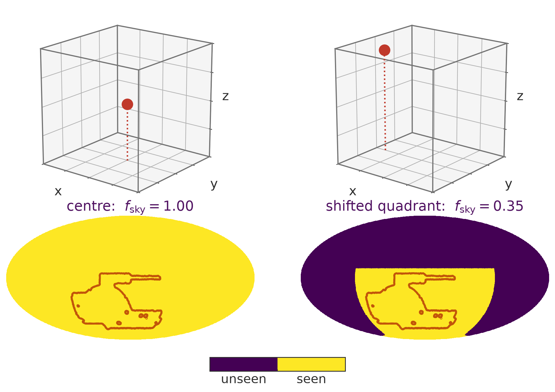
Scientific goal: applications to CMB × LSS with CMB lensing
Removing computational bottlenecks for Stage IV surveys
Early Universe · inflation
Spatial variability for the CMB
Late Universe · dark matter
Explicit field-level inference for large-scale structure




Thank you
\[ f(\theta,\varphi) = \sum_{\ell=0}^{\infty} \sum_{m=-\ell}^{\ell} a_{\ell m}\, Y_\ell^m(\theta,\varphi) \]
\[ C_\ell = \frac{1}{2\ell+1} \sum_{m=-\ell}^{\ell} |a_{\ell m}|^2 \]
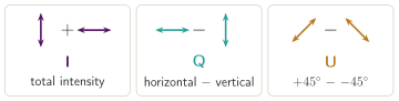
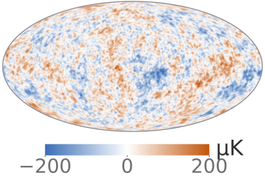 I

spin-0
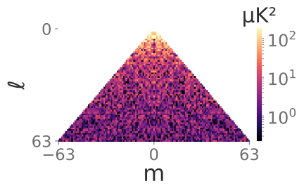 \(|a^T_{\ell m}|^2\)
 Q
spin-2
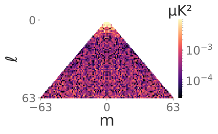 \(|a^E_{\ell m}|^2\)
 U
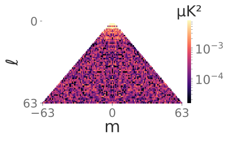 \(|a^B_{\ell m}|^2\)
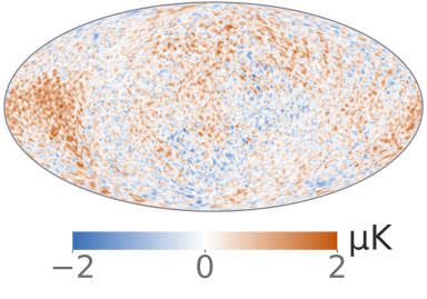
Credit: ESA / Planck Collaboration · Planck 2018 SMICA maps (inpainted), \(I\), \(Q\), \(U\)
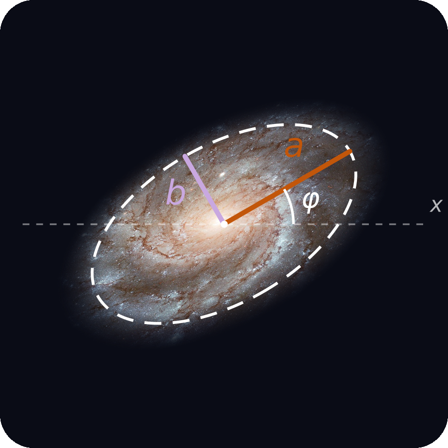
M101: NASA / ESA / Hubble (STScI-PRC2006-10a)
ellipticity \[e = e_1 + i\,e_2 = \frac{a-b}{a+b}\,e^{2i\varphi}\]
shear in a pixel \[\hat\gamma_1 = \frac{\sum_k w_k\,e_{1,k}}{\sum_k w_k}, \qquad \hat\gamma_2 = \frac{\sum_k w_k\,e_{2,k}}{\sum_k w_k}\]
From \(\kappa\) to \(\gamma\)
\[ \gamma^E_{\ell m} = -\sqrt{\frac{(\ell+2)(\ell-1)}{\ell(\ell+1)}}\;\kappa_{\ell m}, \qquad \gamma^B_{\ell m} = 0 \] \[ \gamma_1 + i\gamma_2 = \sum_{\ell m} \gamma^E_{\ell m}\;{}_2Y_{\ell m} \]
From \(\gamma\) back to \(\kappa\)
\[ \kappa_{\ell m} = -\sqrt{\frac{\ell(\ell+1)}{(\ell+2)(\ell-1)}}\;\gamma^E_{\ell m} \]
convergence κ
shear γ1
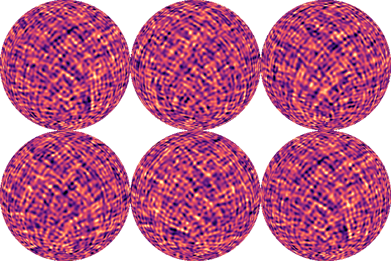
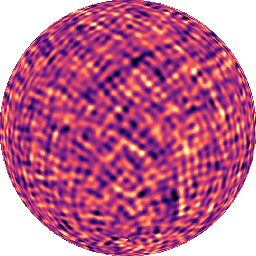
shear γ2

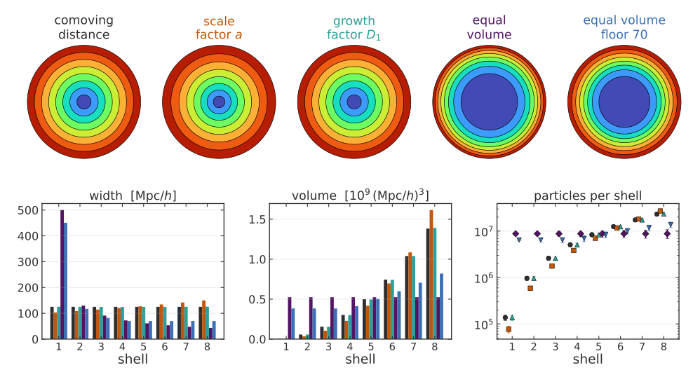
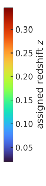
10 shells, one redshift per shell
10 shells, drifted
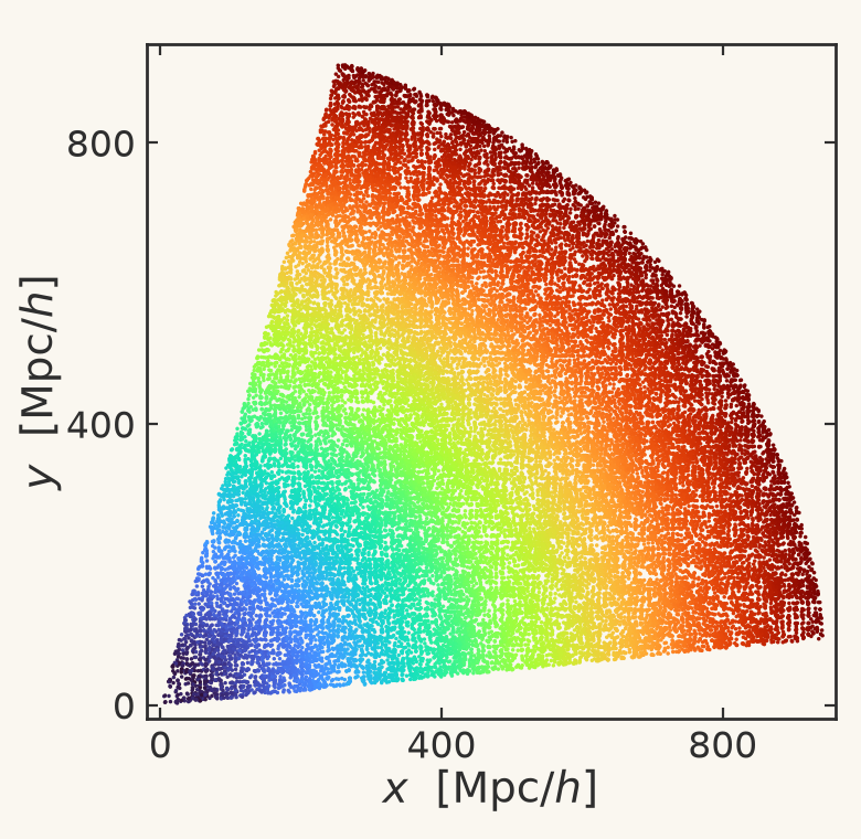
40 shells, one redshift per shell
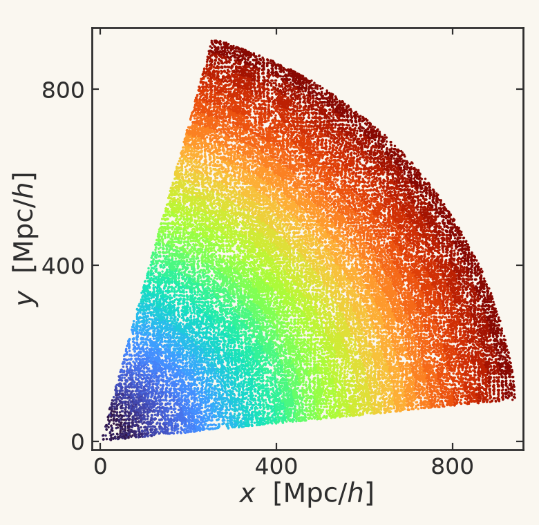
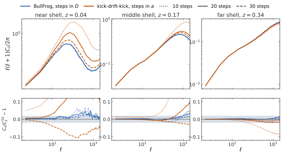
\[a_{\mathrm{c}} = a\big(\chi = \lVert \mathbf{x} - \mathbf{x}_{\mathrm{obs}} \rVert\big), \qquad \mathbf{x}(a_{\mathrm{c}}) = \mathbf{x}(a_i) + \boldsymbol{\pi}\,\big[D(a_{\mathrm{c}}) - D(a_i)\big]\]
\(a_i\): scale factor of the shell, \(a_{\mathrm{c}}\): scale factor at which the particle crosses the lightcone, \(\boldsymbol{\pi} = \mathrm{d}\mathbf{x}/\mathrm{d}D\): BullFrog momentum
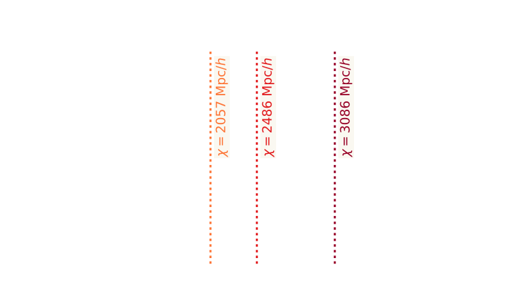
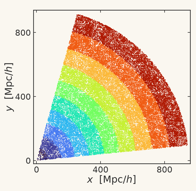
Interpolating the particles onto the observer’s lightcone
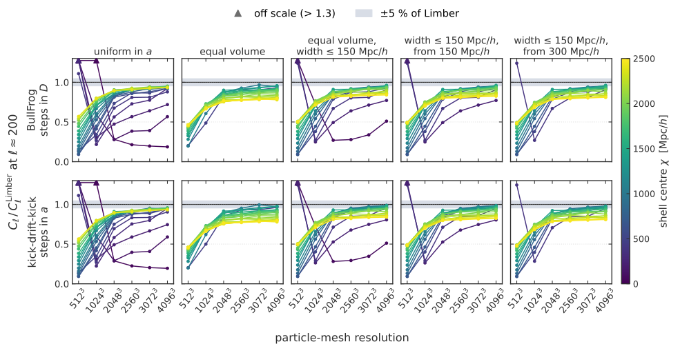
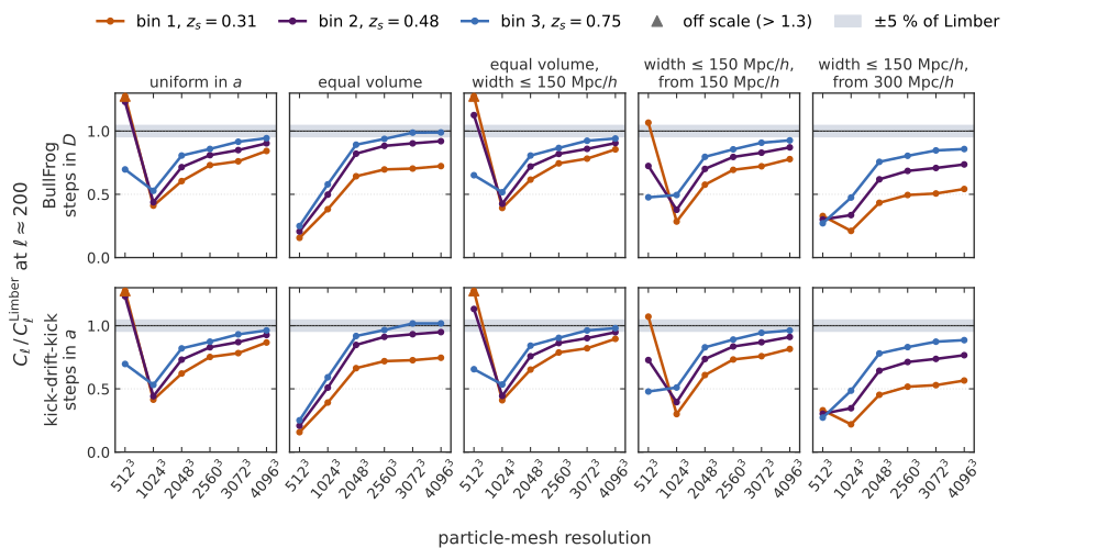
Each particle is drifted to the scale factor at which it crosses the lightcone
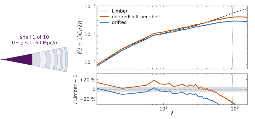
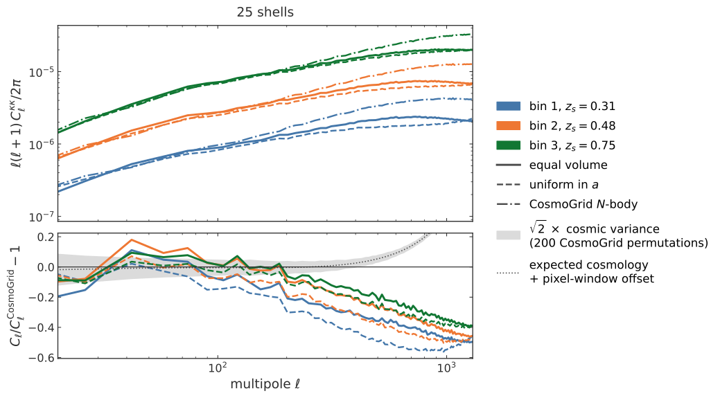
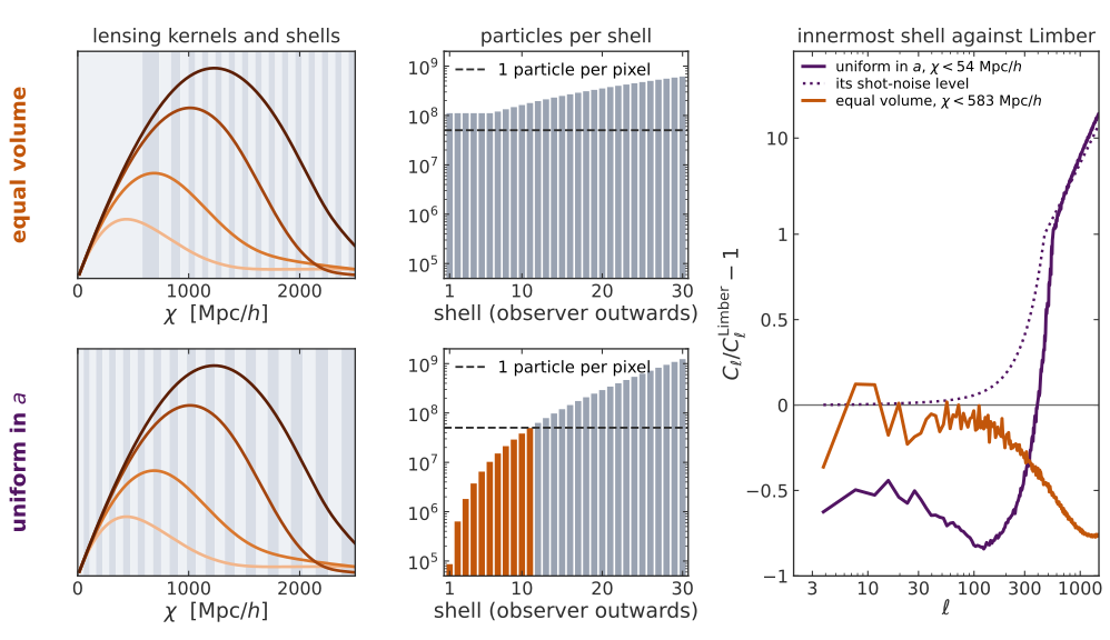
Removes the single-redshift bias of wide shells: 17 % on the first equal-volume shell
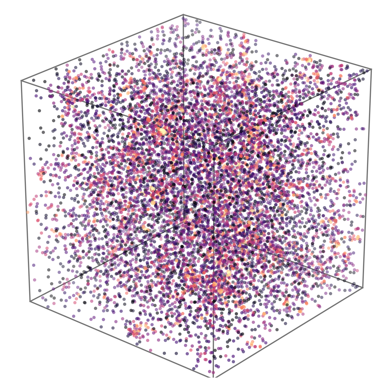
evolved particles
⟶
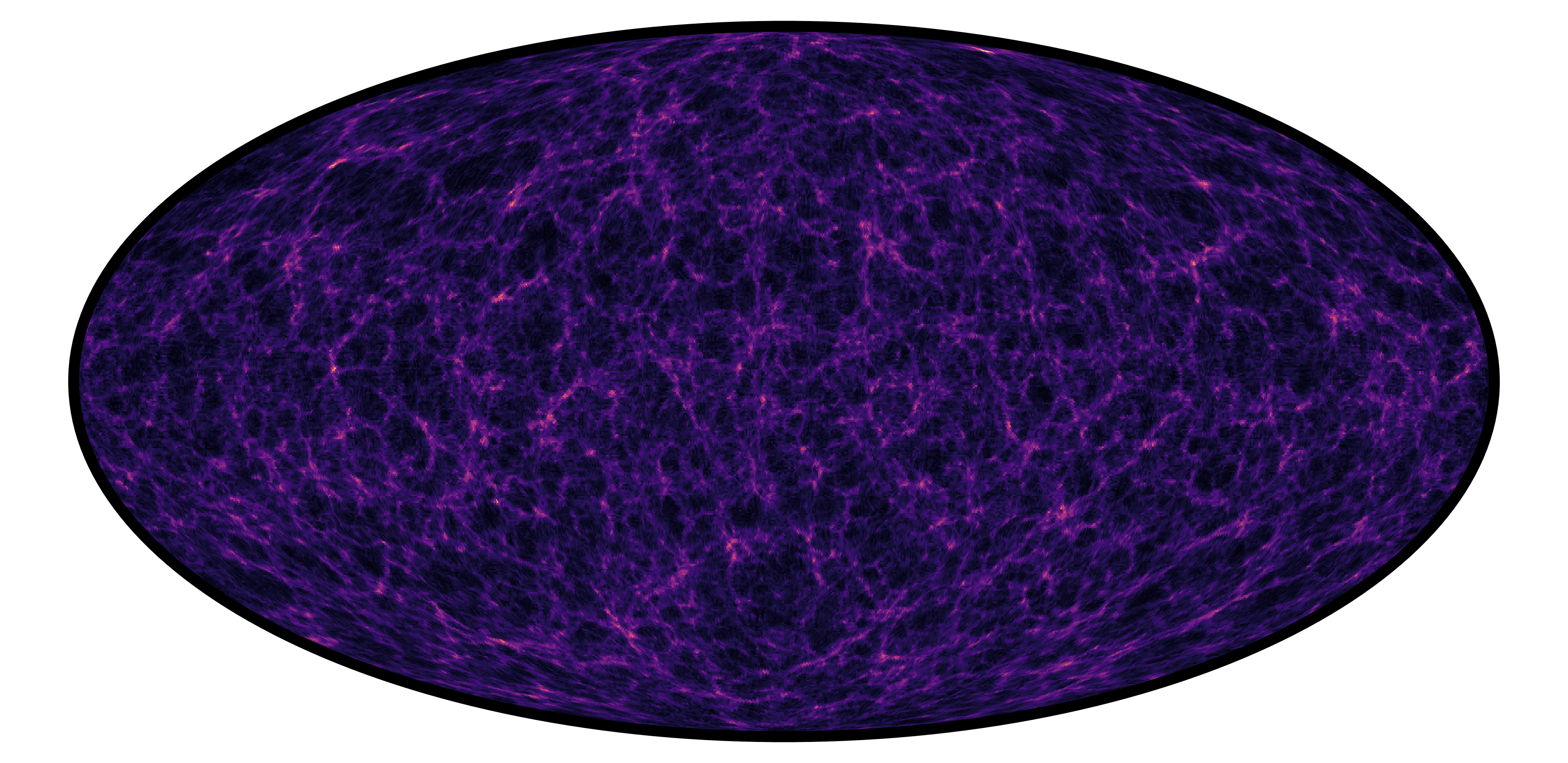
one HEALPix shell
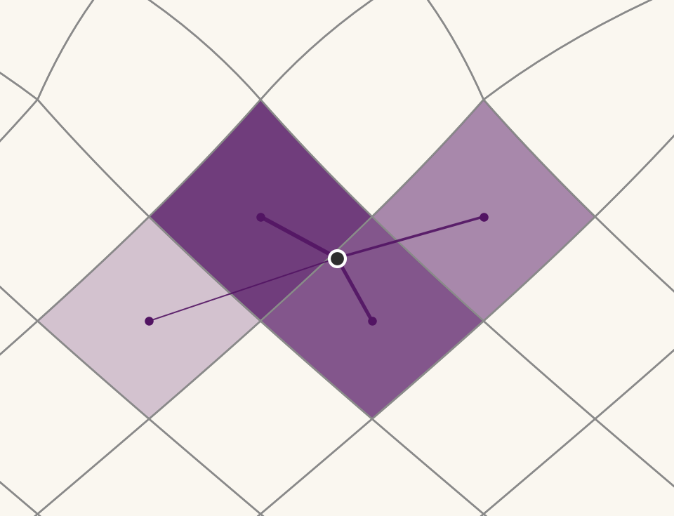
Four pixels, weighted by the position between their centres: get_interp_weights, implemented in jax-healpy
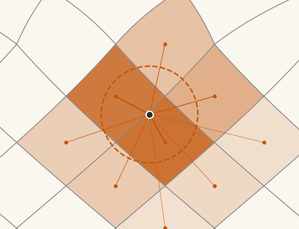
The pixel and its eight neighbours (get_all_neighbours, implemented in jax-healpy), weighted by a Gaussian kernel of adjustable width
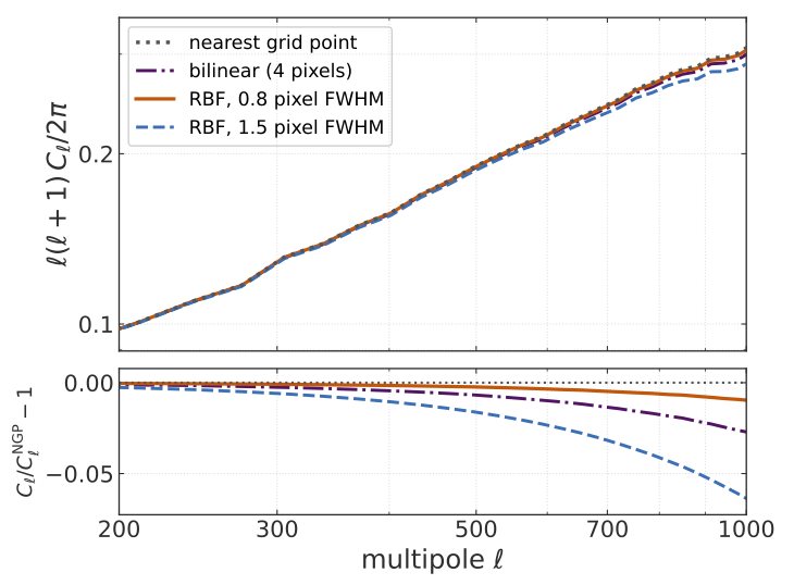
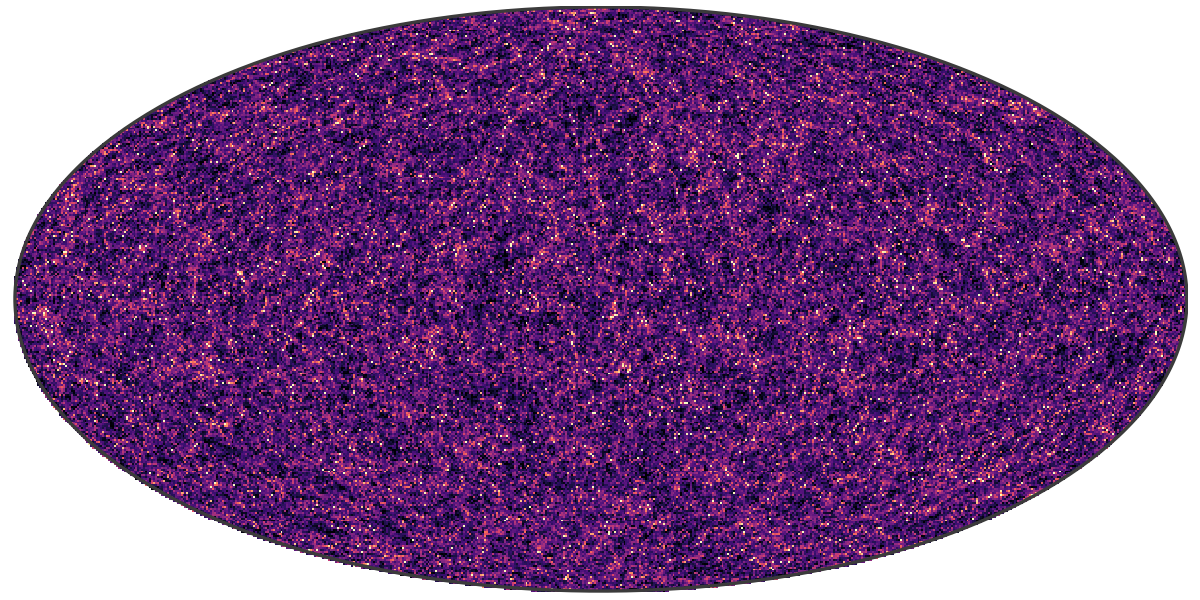
map2alm
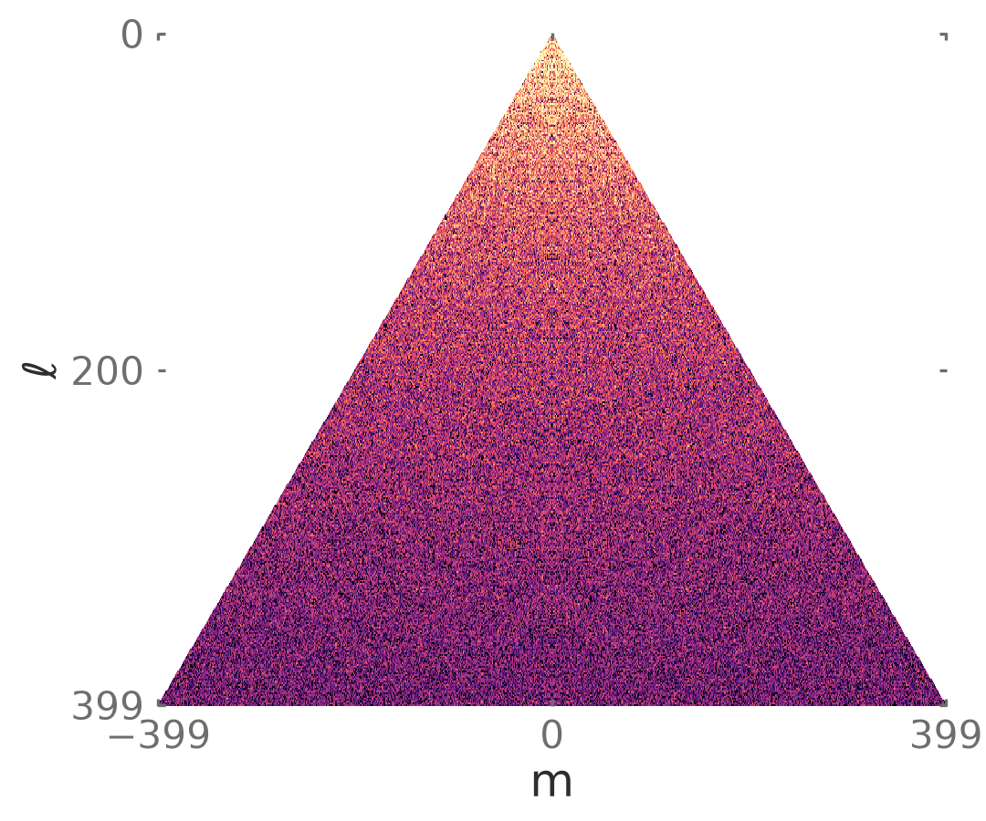
× \(T_\ell\)
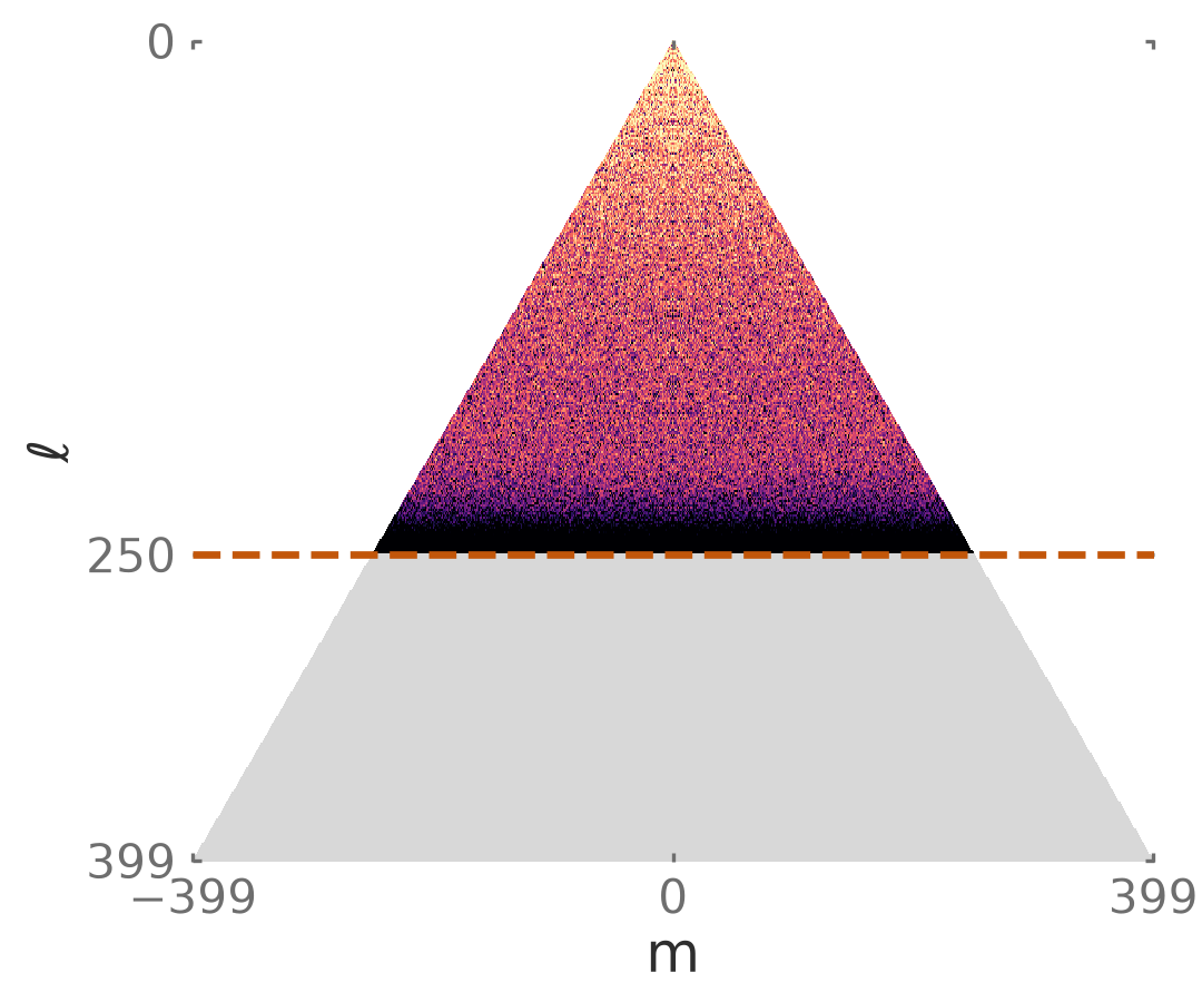
alm2map
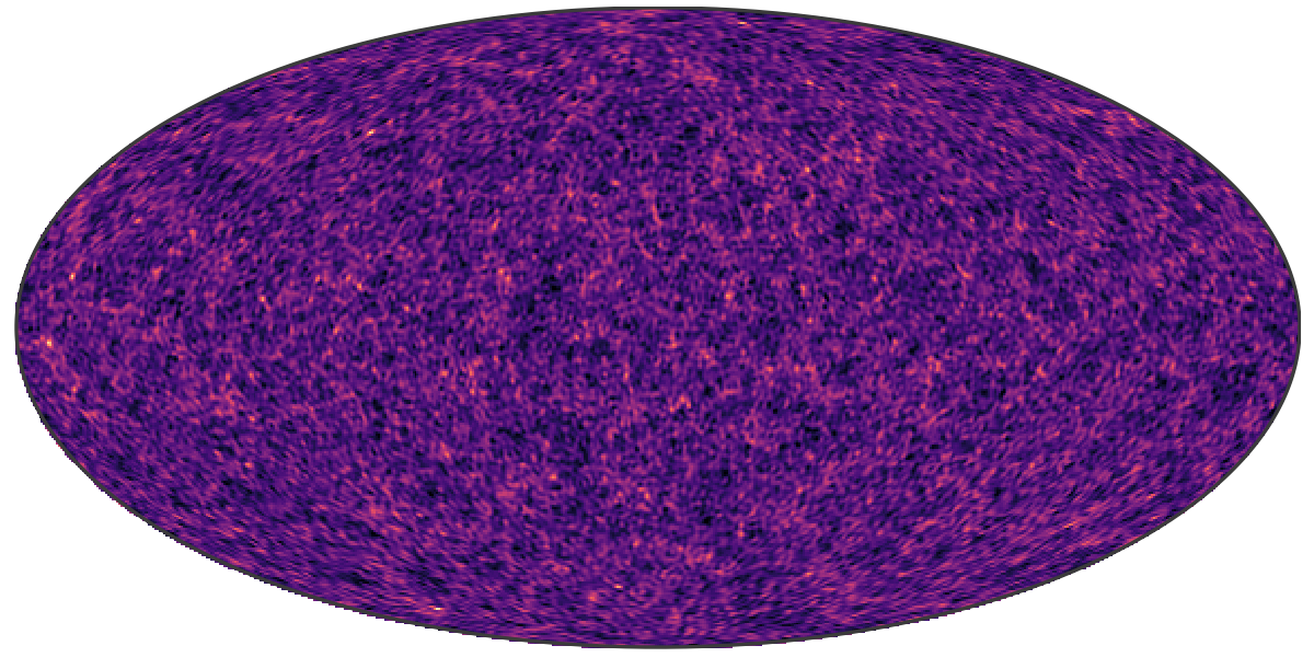
\[T_\ell = \begin{cases} 1, & \ell \le \ell_\mathrm{cut} - \ell_\mathrm{width} \\ \tfrac12\left(1 + \cos \pi x\right), & \ell_\mathrm{cut} - \ell_\mathrm{width} < \ell < \ell_\mathrm{cut} \\ 0, & \ell \ge \ell_\mathrm{cut} \end{cases}\]
\[x = \frac{\ell - (\ell_\mathrm{cut} - \ell_\mathrm{width})}{\ell_\mathrm{width}}\]
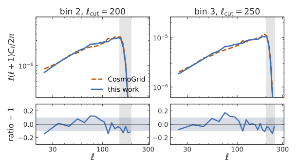
Tersenov, Guerrini, Starck & Kilbinger (2026), arXiv:2609.09131
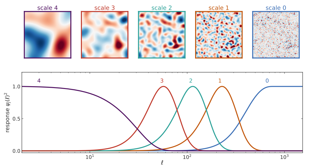
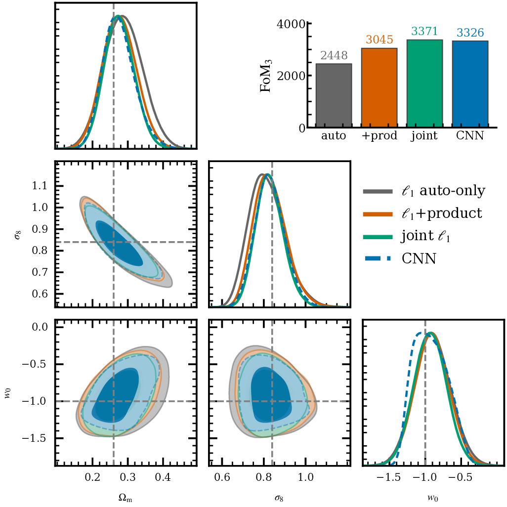
Ajani et al. (2021), arXiv:2101.01542; Tersenov et al. (2026), in prep.
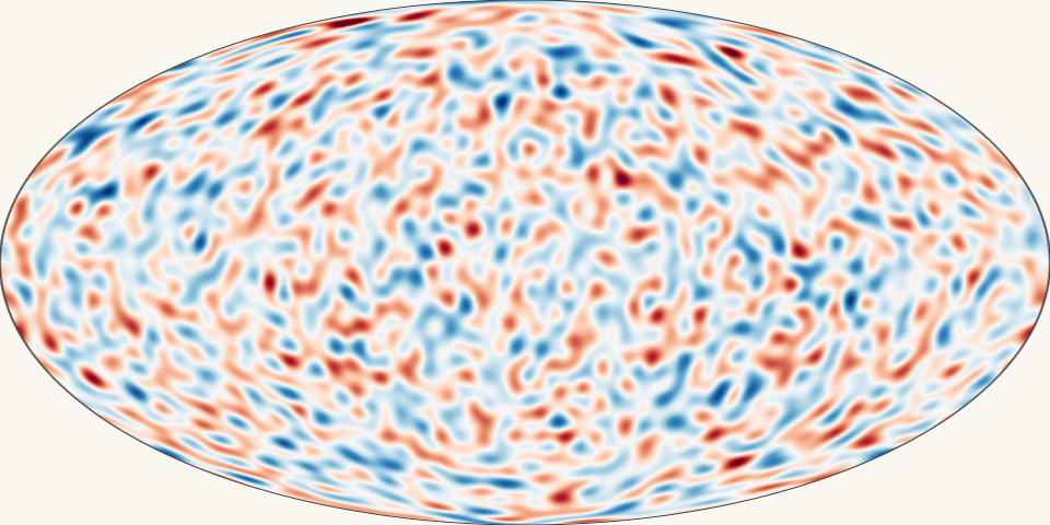
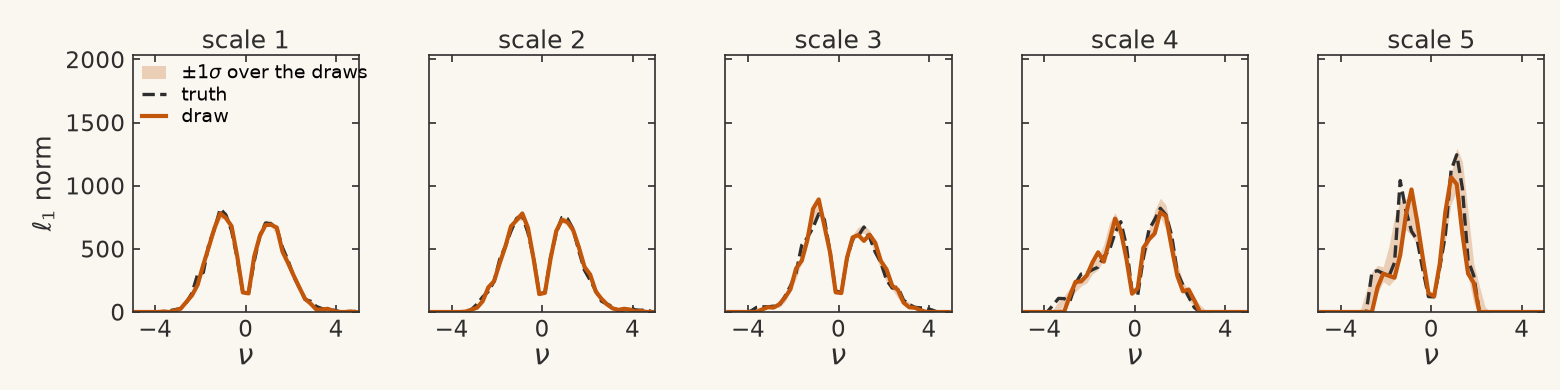
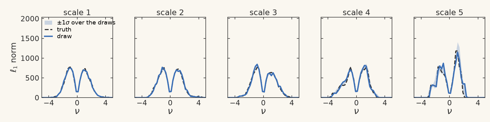
truth
posterior draws
standard deviation
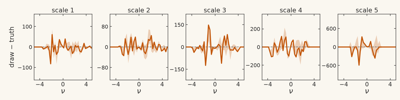
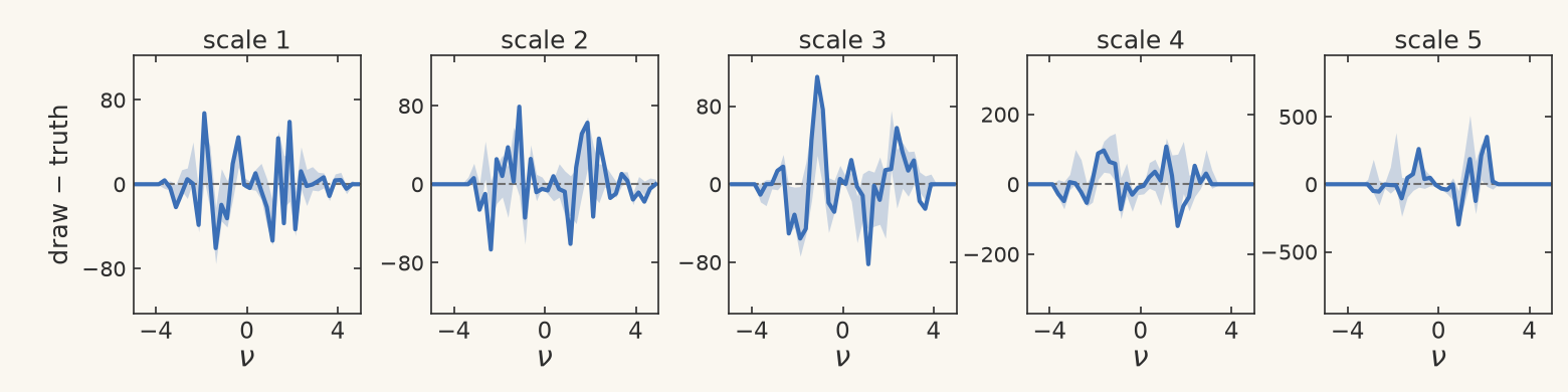
truth − draw
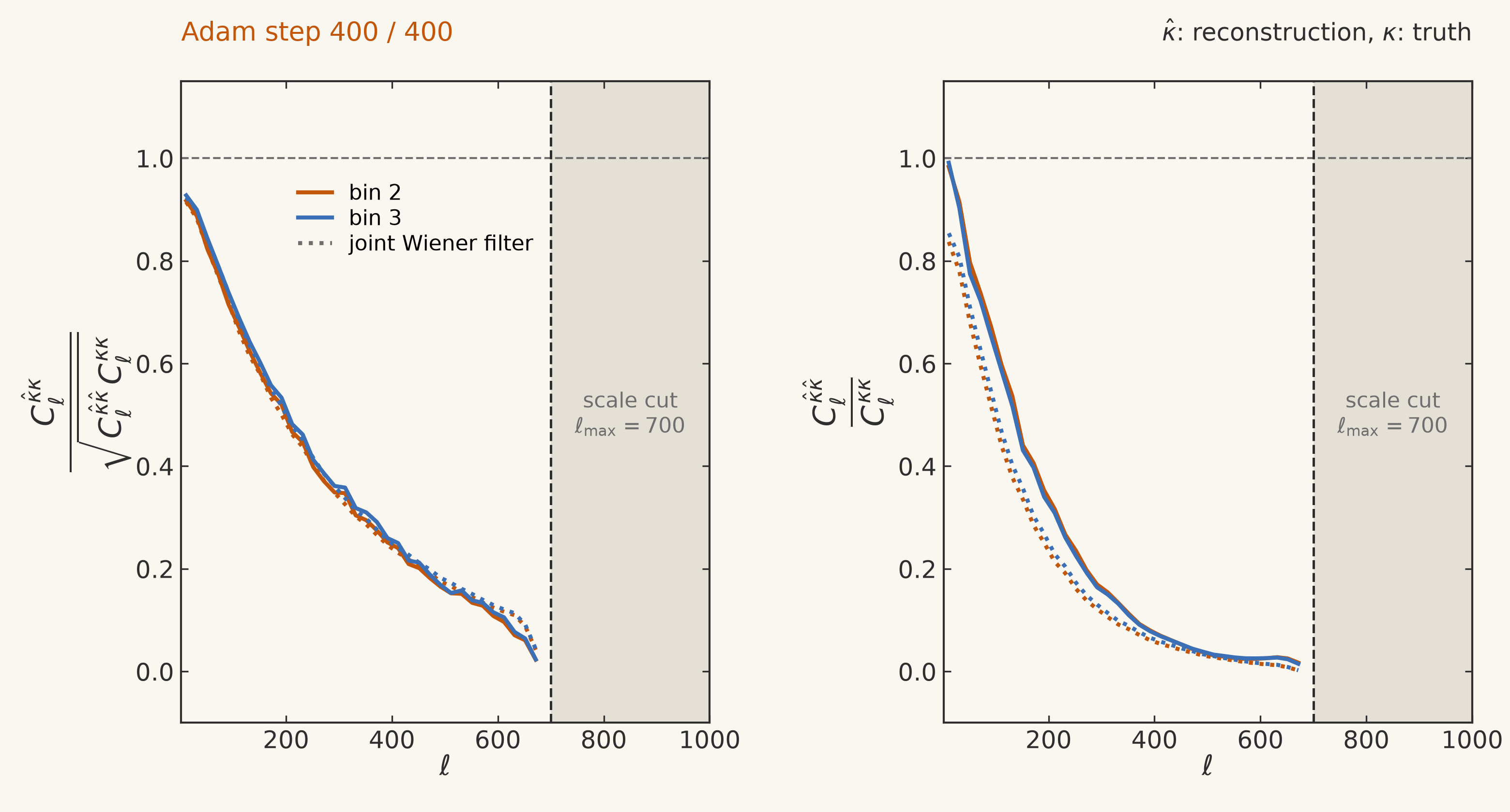
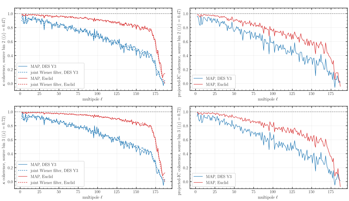
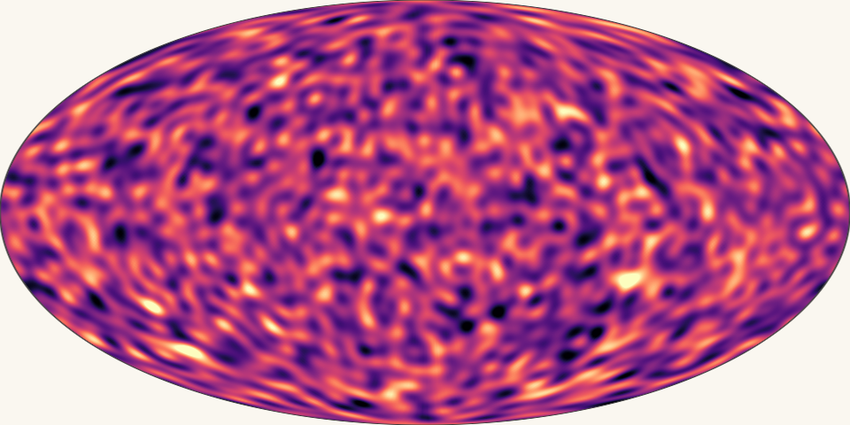
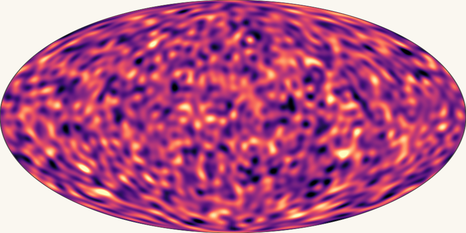
bin 2
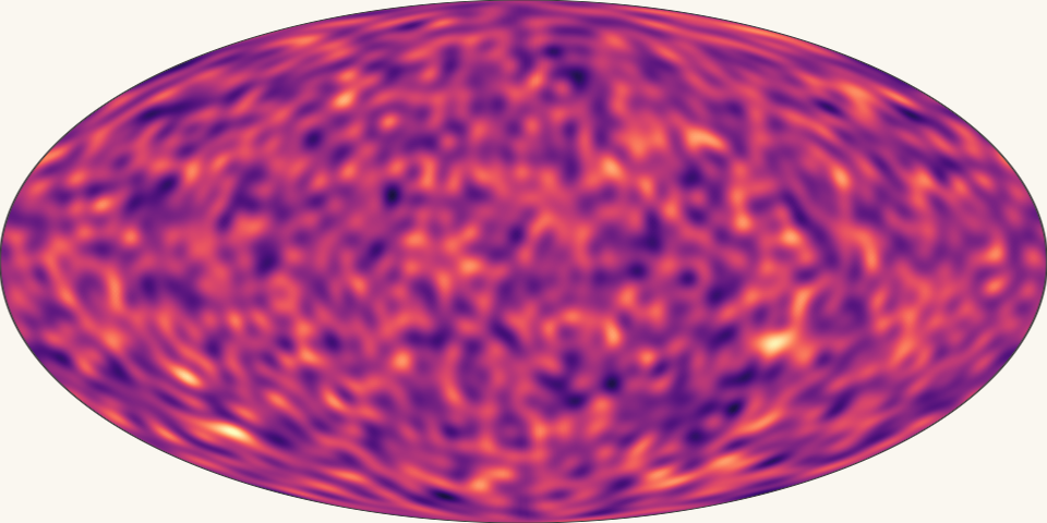
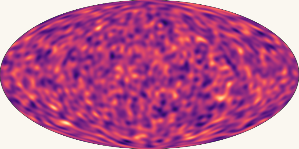
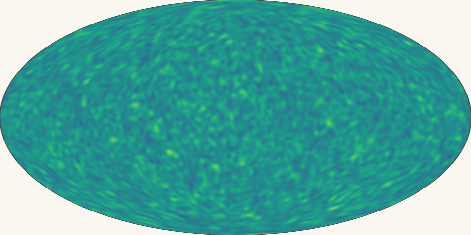
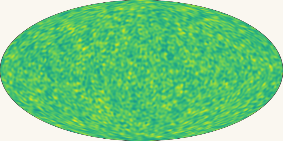
bin 3
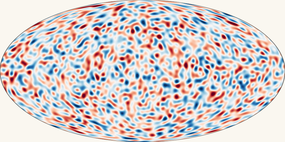
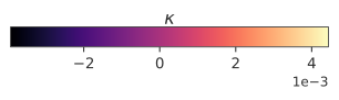
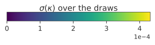
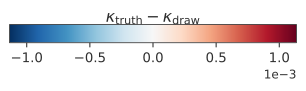
| MCLMC on one A100: \(128^3\) initial conditions and \((\Omega_c, \sigma_8)\) | Wall time |
|---|---|
| Compiling the tuning step | 12 min |
| Tuning the step size and momentum decoherence: 300 steps | 1 h 32 min |
| Compiling the sampler | 1.5 min |
| Sampling: 10 batches of 10 draws, one draw every 5 steps | 15.5 min per batch |
| Total | ≈ 4 h 20 min |
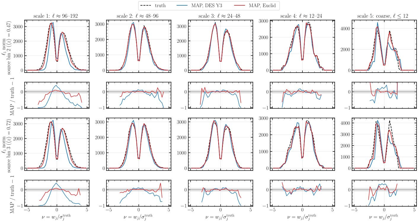
bin 2
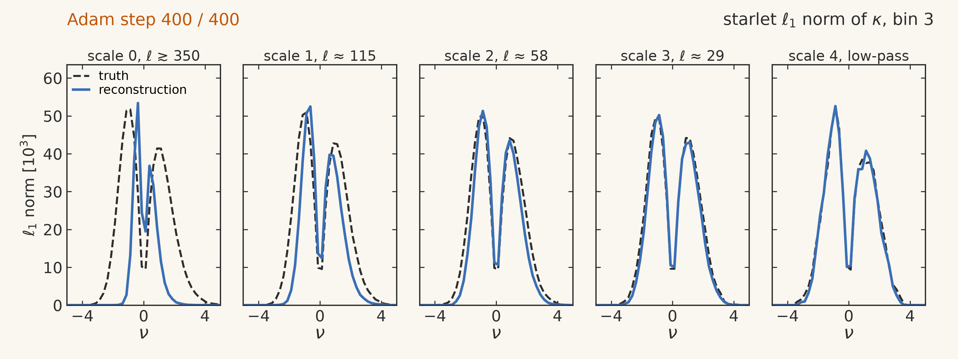
ℓ₁ norm
bin 2
draw − truth
bin 3
ℓ₁ norm
bin 3
draw − truth
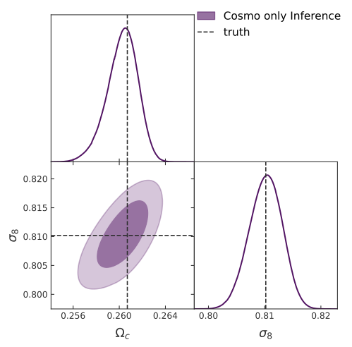
| NUTS, initial conditions at the truth | |
|---|---|
| Warmup | 100 iterations |
| Sampling | 10 batches of 10 draws |
| \(\Omega_c\) | \(0.2603 \pm 0.0013\) (truth 0.2607) |
| \(\sigma_8\) | \(0.8102 \pm 0.0025\) (truth 0.8102) |
| Wall time | 4 h 56 min |
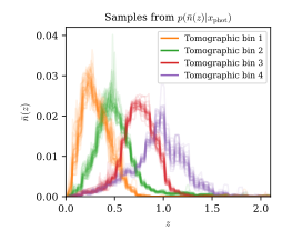
Jeffrey et al. (2024), arXiv:2403.02314; Cordero et al. (2022)
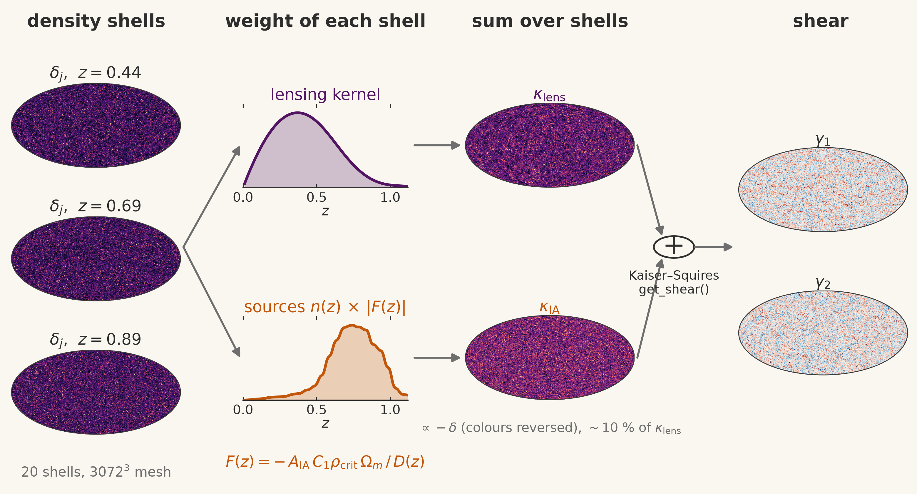
Tsaprazi et al. (2022), arXiv:2112.04484
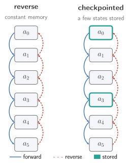
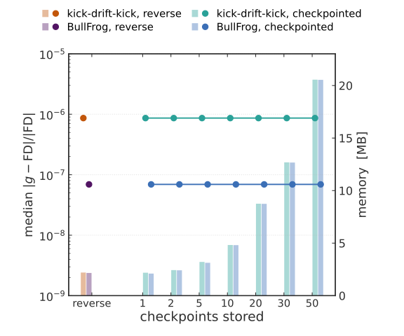

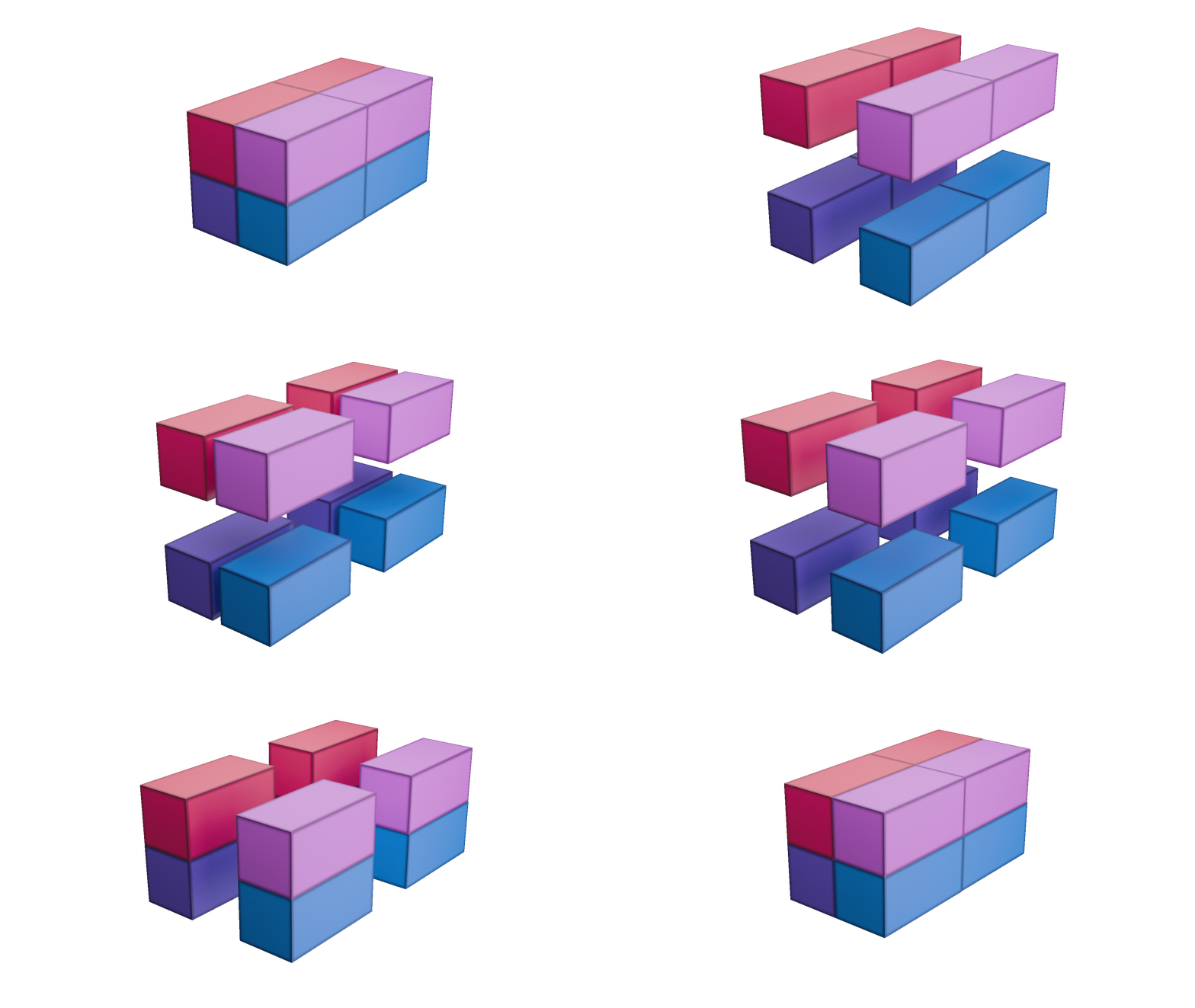
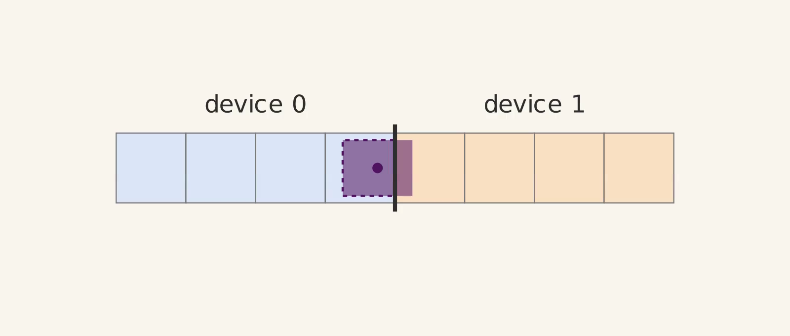
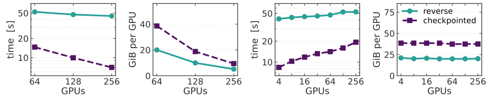
Jean Zay, IDRIS
NVIDIA H100 GPUs
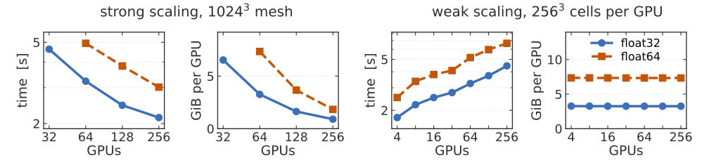
Performance of the forward model
Performance of the gradient
Jean Zay, IDRIS
NVIDIA H100 GPUs
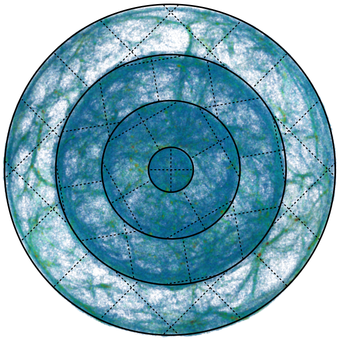
Sgier et al. (2021), arXiv:2007.05735