Generative AI with JAX

Wassim Kabalan

2025-10-01

Outline for This Presentation

• Introduction to Generative AI
  Understand the mathematical meaning of generating data
  
  
• Deep dive into Generative Models
  Explore the different framework and state of the art ways of generative AI
  
  
• JAX eco system
  Learn core JAX transforms (jit, vmap, grad) and Flax tooling
  
  
• Hands on tutorial
  
  Explore how generative AI can be used for cosmological inference

This workshop covers three main sections: first, we’ll explore different generative AI models and their mathematical properties. Then we’ll introduce JAX and its ecosystem for high-performance computing. Finally, we’ll apply these techniques to real cosmology problems with hands-on notebooks.

What is Generative AI?

What does “generate” mean?

Generated faces example

Key Idea: Generative AI

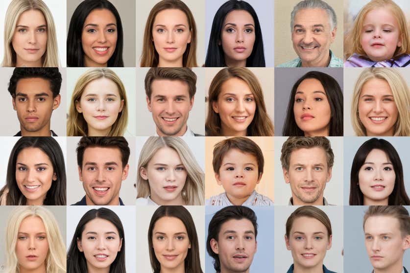
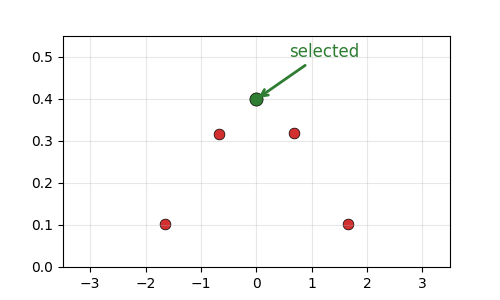
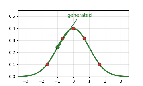
• Generative AI is about learning the underlying distribution \(p(\text{data})\) and sampling from it to generate images.
• The output of a generative model is a new data point.
• Generative is intrinsically related to probability distributions.

Generative AI is about learning probability distributions over data. Unlike discrete lookup tables, generative models learn continuous distributions and can sample entirely new data points. The key is modeling \(p(\text{data})\) accurately enough to generate realistic samples.

Generative Models

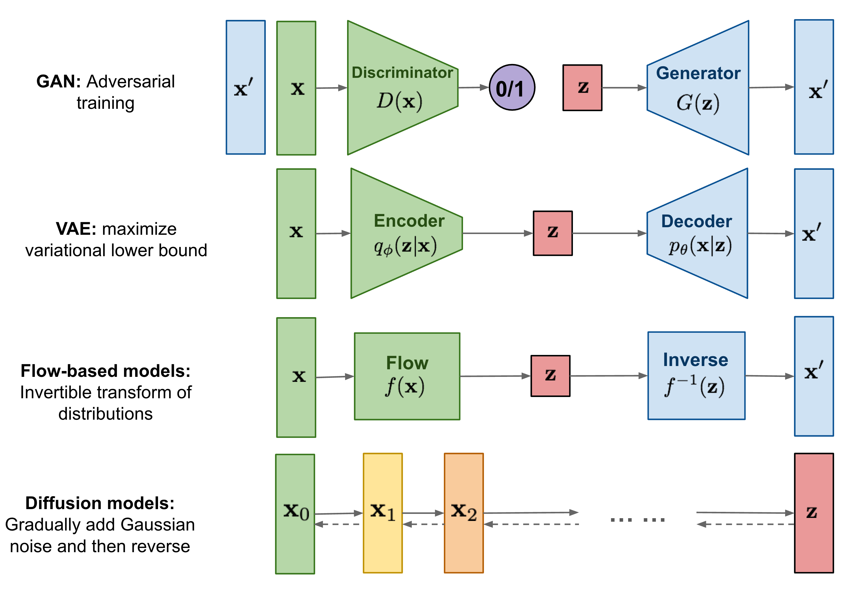
Generative Adversarial Networks (GANs)

GAN Architecture

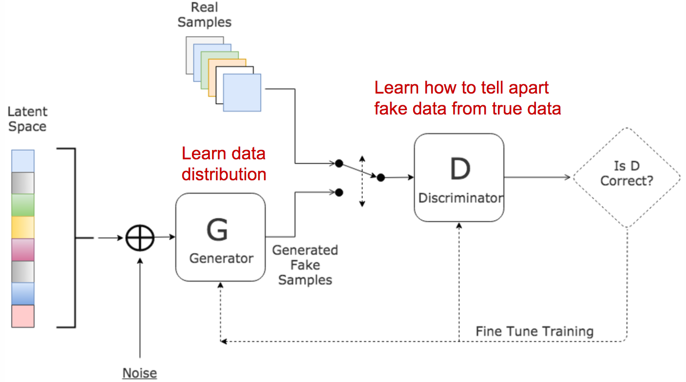
\[\min_G \max_D \mathbb{E}_{x\sim p_\text{data}}[\log D(x)] + \mathbb{E}_{z\sim p(z)}[\log(1 - D(G(z)))]\]

• Loss function
  • Generator: produces samples G(z) to fool D
  • Discriminator: estimates real vs fake probability D(·)

Advantages and Limitations

• Advantages: sharp samples; flexible implicit modeling; no explicit likelihood.
• Limitations: unstable training; mode collapse; sensitive to architecture and tricks.

Limitations with GANs

Unstable learning

Nash equilibrium illustration

Mode collapse

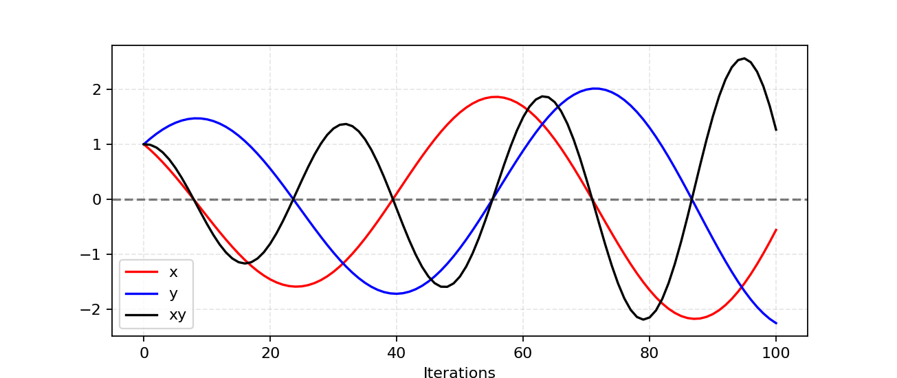
Mode collapse

Vanishing gradients

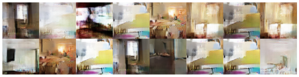
Vanishing gradients

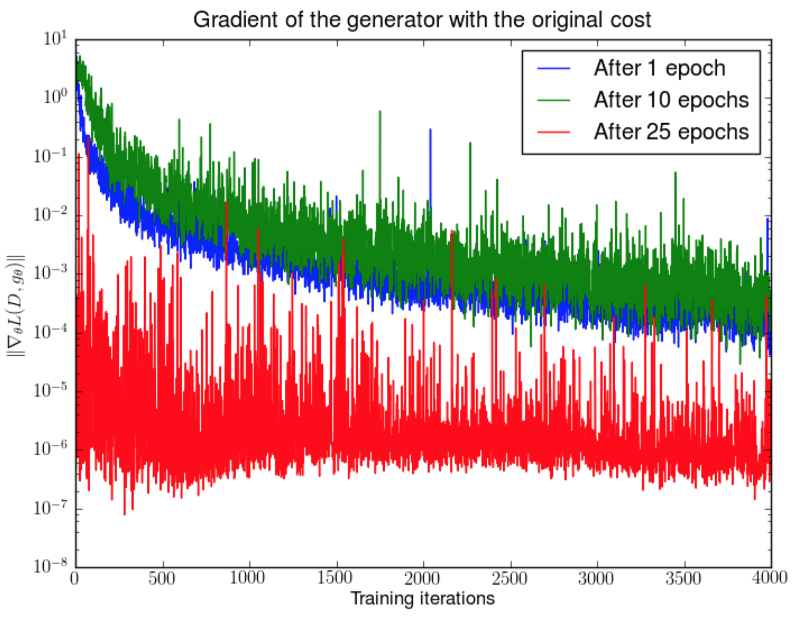
Some possible solutions

• Use WGAN for more stable training and stronger gradients.
• Add gradient penalty (WGAN-GP) to keep the critic smooth.

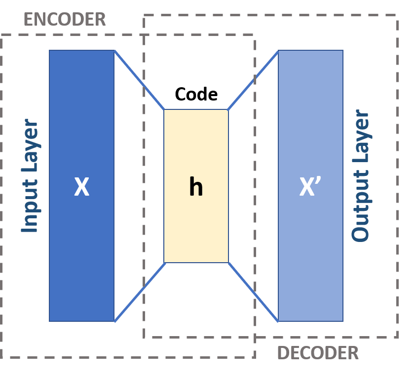
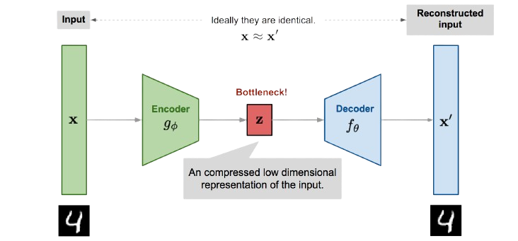
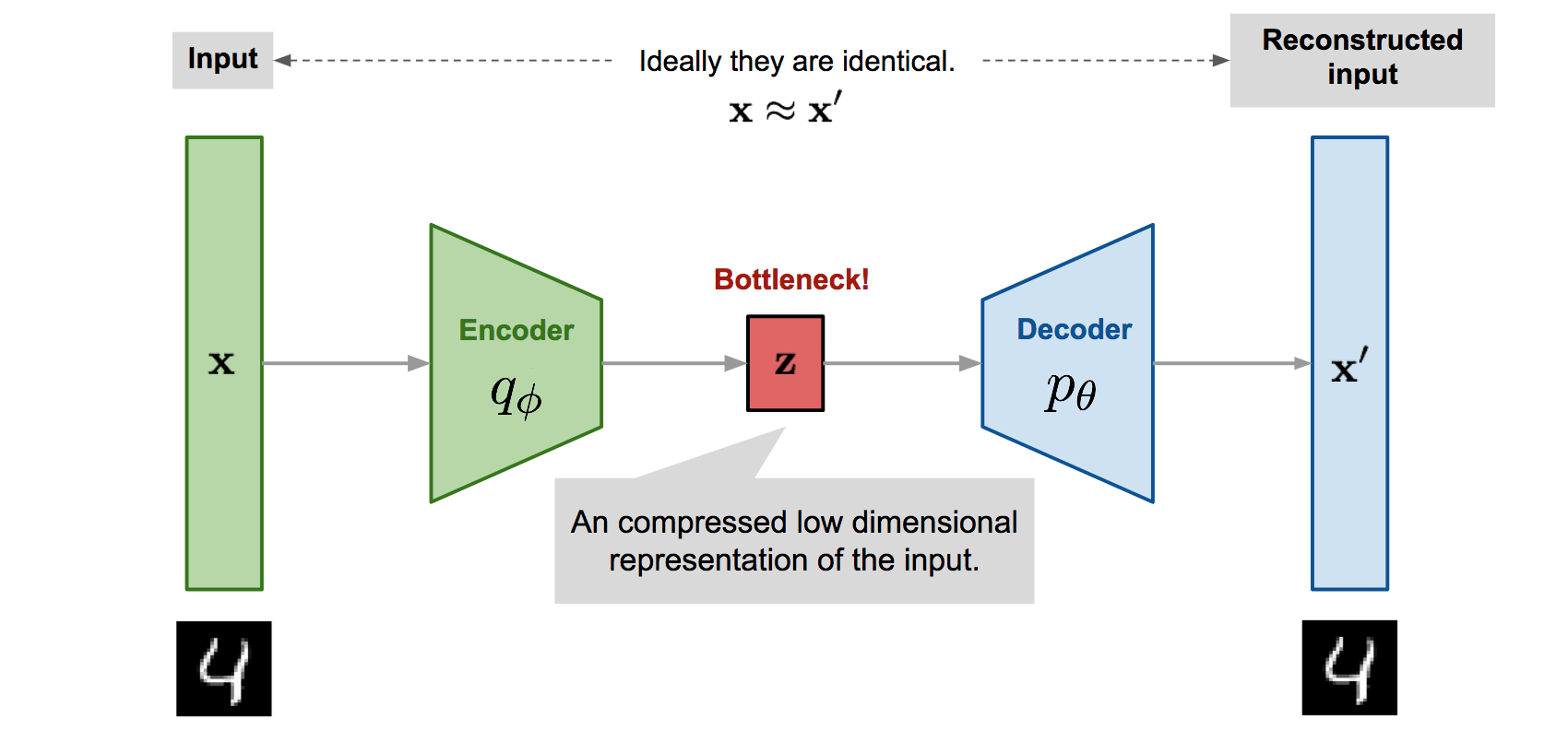
Variational Autoencoders (VAEs)

Autoencoder architecture

VAE architecture

VAE takeaways

• VAE learn optimal compression into the latent space
• Represents a dataset by an easy to sample gaussian distribution
• Compared to GAN gives a better access to probability distribution
• Produces blurrier images than GANs

VAE paper title

Evidence Lower Bound (ELBO):

\[\mathcal{L} = \mathbb{E}_{q_\phi(z|x)}[\log p_\theta(x|z)] - \text{KL}(q_\phi(z|x)\|p(z))\]

• Reconstruction: decoder quality
• KL Divergence: latent regularization

Reparameterization trick: \[z = \mu + \sigma \odot \epsilon, \quad \epsilon \sim \mathcal{N}(0,I)\]

VAEs use an encoder-decoder architecture with a probabilistic latent space. The encoder outputs mean and log-variance for a Gaussian posterior. The reparameterization trick allows backpropagation through the stochastic sampling. The ELBO balances reconstruction quality against matching a prior distribution, typically standard normal.

VAE — Why KL matters (β-VAE)

Without KL regularization:

Unregularized

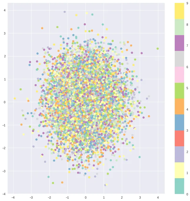
Latent space is unstructured

With KL regularization:

Regularized

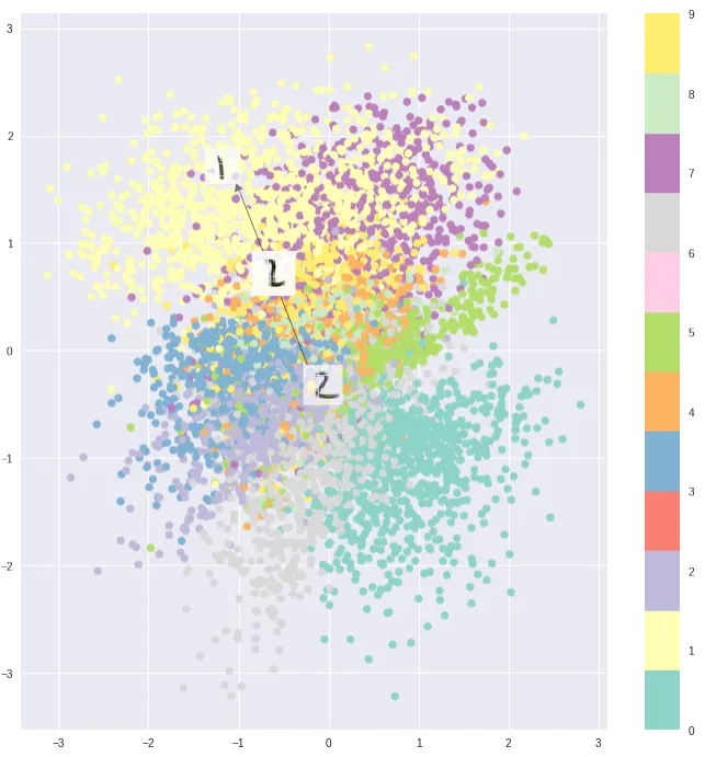
Organized, continuous latent space

β-VAE objective:

\[\mathcal{L}_\beta = \mathbb{E}[\log p_\theta(x|z)] - \beta \cdot \text{KL}(q_\phi(z|x)\|p(z))\]

• \(\beta > 1\): More disentanglement, less reconstruction
• \(\beta < 1\): Better reconstruction, less structure
• Limitation: Gaussian prior can bias toward simpler shapes

The KL term is crucial for organizing the latent space. Without it, the encoder can map inputs to arbitrary regions making interpolation meaningless. Beta-VAE introduces a hyperparameter β to control the tradeoff between reconstruction quality and latent space disentanglement. Higher β encourages more interpretable latent dimensions but may reduce reconstruction fidelity.

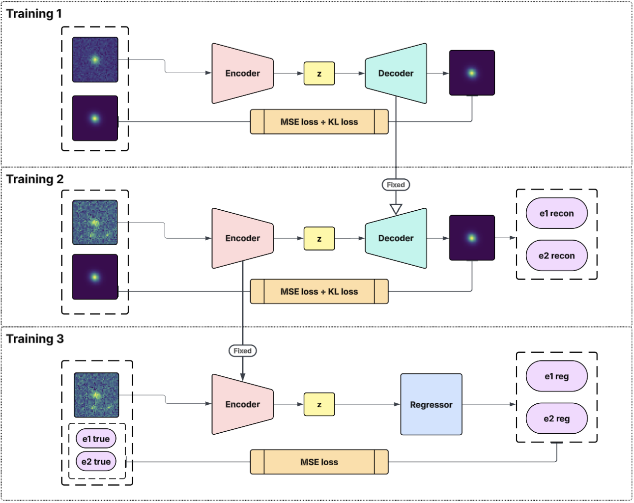
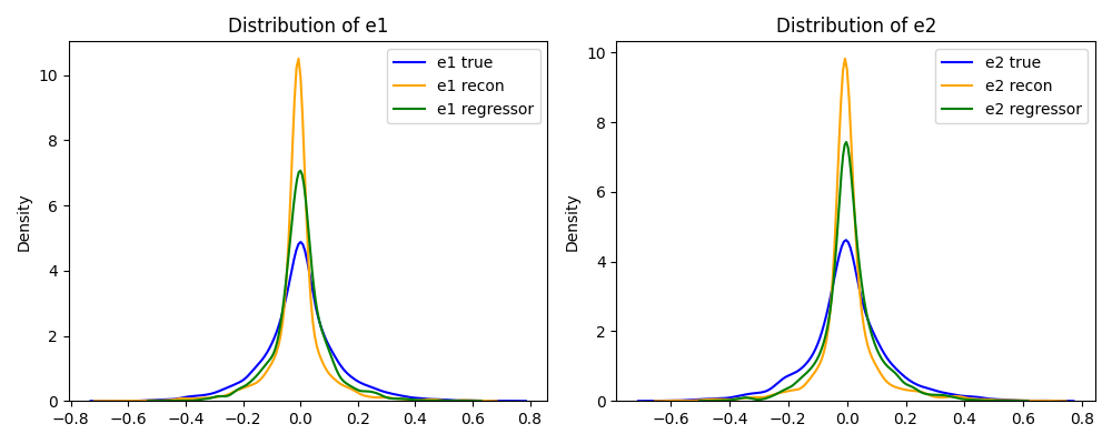
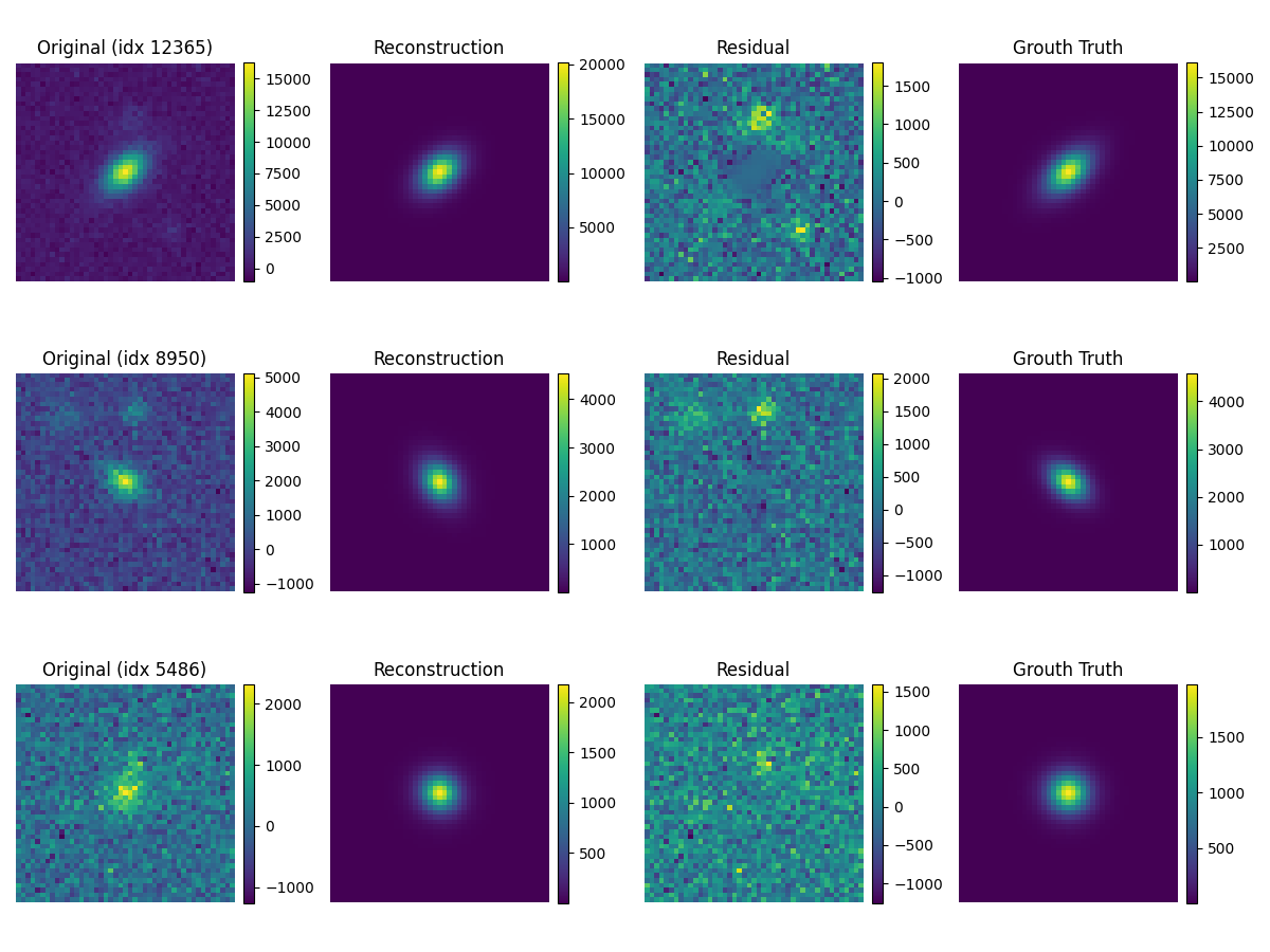
VAE in Cosmology (Deblending)

Binh Nguyen

Deblender architecture

Distribution e1/e2

Reconstructions

In cosmology, VAEs are used for galaxy deblending and morphology analysis. The latent representation can compress galaxy images efficiently. However, the Gaussian prior assumption can bias reconstructions toward rounder shapes, which is problematic for weak lensing studies that need accurate ellipticity measurements. This motivates using more flexible priors like normalizing flows.

Normalizing Flows (Flow-based Generative Models)

Flow intuition (© Lilian Weng, Lil’Log)

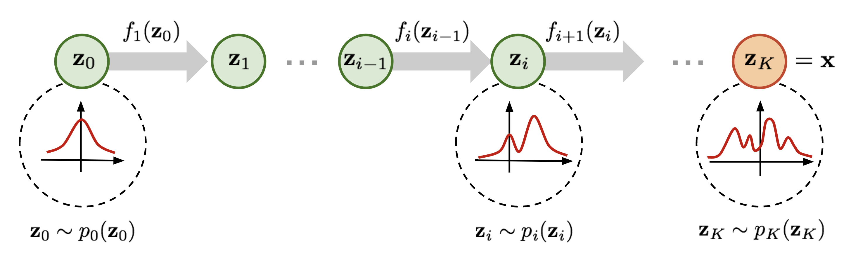
Mappings: \(f(x) \to y\), \(g(y) = z\); \(z = g_{\theta}(x) = g_K \circ \cdots \circ g_1(x)\)

Log-likelihood

\[\log p_{\theta}(x) = \log p_Z\big(g_{\theta}(x)\big) + \sum_{k=1}^{K} \log \left|\det J_{g_k}\right|\]

Rezende & Mohamed (2015)

In short

• Gaussianize data: \(z = g_{\theta}(x) \approx \mathcal{N}(0, I)\).
• Exact likelihood: \(\log p_{\theta}(x) = \log p_Z(z) + \sum_k \log|\det J_{g_k}|\).
• Generate via inverse: \(x = f_{\theta}(z)\), \(z \sim p_Z\).

Flows learn an invertible transform mapping a simple base \(p_Z\) (e.g., \(\mathcal{N}(0,I)\)) to the data distribution. Training maximizes the exact likelihood via the change-of-variables formula with tractable log-determinants.

Coupling Layers : Forward vs Inverse

Coupling layer computation graph

Forward (x → y)

1. Split \(x=(x_a, x_b)\) by mask.
2. Conditioning network on kept half: \((s, t) = \text{NN}(x_a)\).
3. Affine update (element-wise):

\[ y_a = x_a, \qquad y_b = x_b \odot e^{s(x_a)} + t(x_a). \]

Inverse (y → x)

Given \((y_a, y_b)\):

1. Recompute \((s, t) = \text{NN}(y_a)\).
2. Invert the affine on the transformed half:

\[ x_a = y_a, \qquad x_b = \big(y_b - t(y_a)\big) \odot e^{-s(y_a)}. \]

Masked Autoregressive Flow (MAF) vs Inverse Autoregressive Flow (IAF)

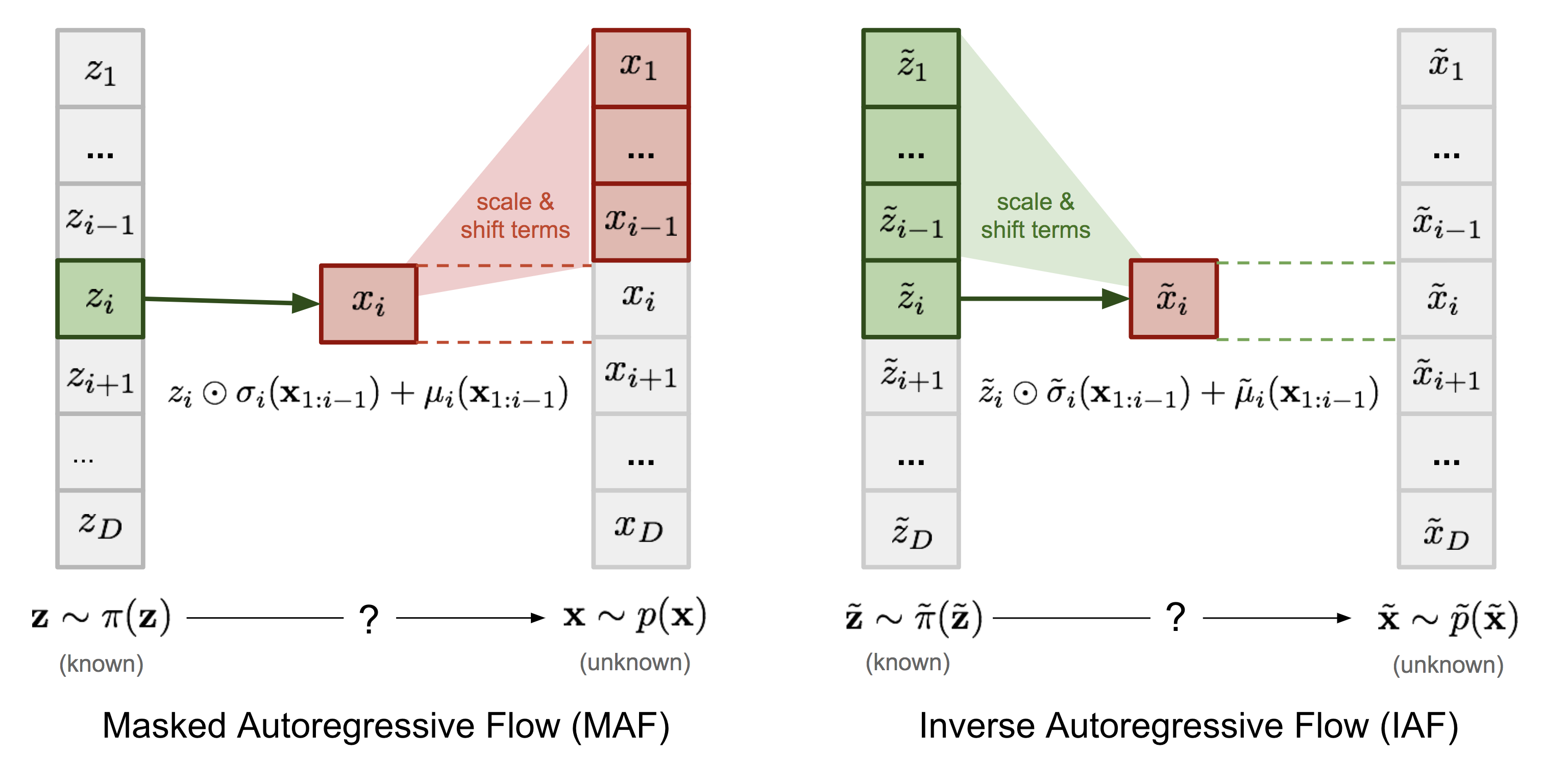
MAF vs IAF comparison

MAF (Masked Autoregressive Flow)

Autoregressive flow where density evaluation is parallel sampling is sequential.

\[ z_i=\frac{x_i-\mu_i(x_{<i})}{\sigma_i(x_{<i})} \]

IAF (Inverse Autoregressive Flow) — fast sampling

Same masked structure but reversed so sampling is parallel (given \(z\)), density is sequential.

\[ x_i=\mu_i(z_{<i})+\sigma_i(z_{<i})\cdot z_i \]

Diffusion Models

DDPM process

Diffusion visualization

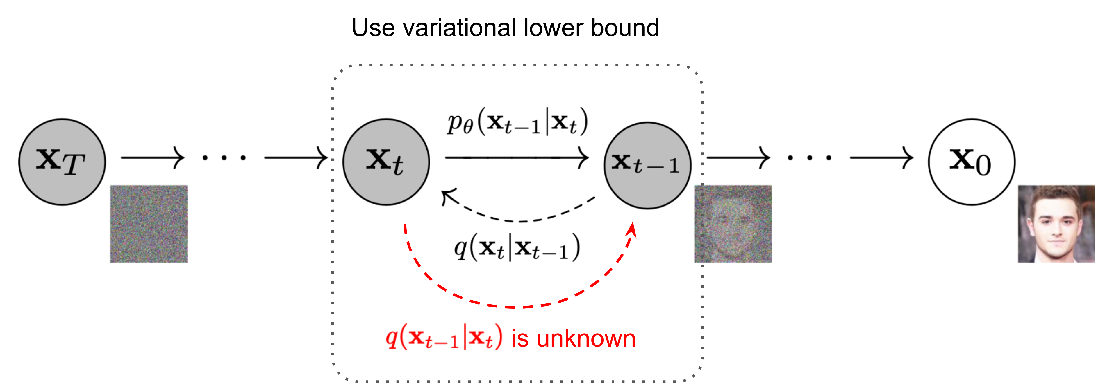
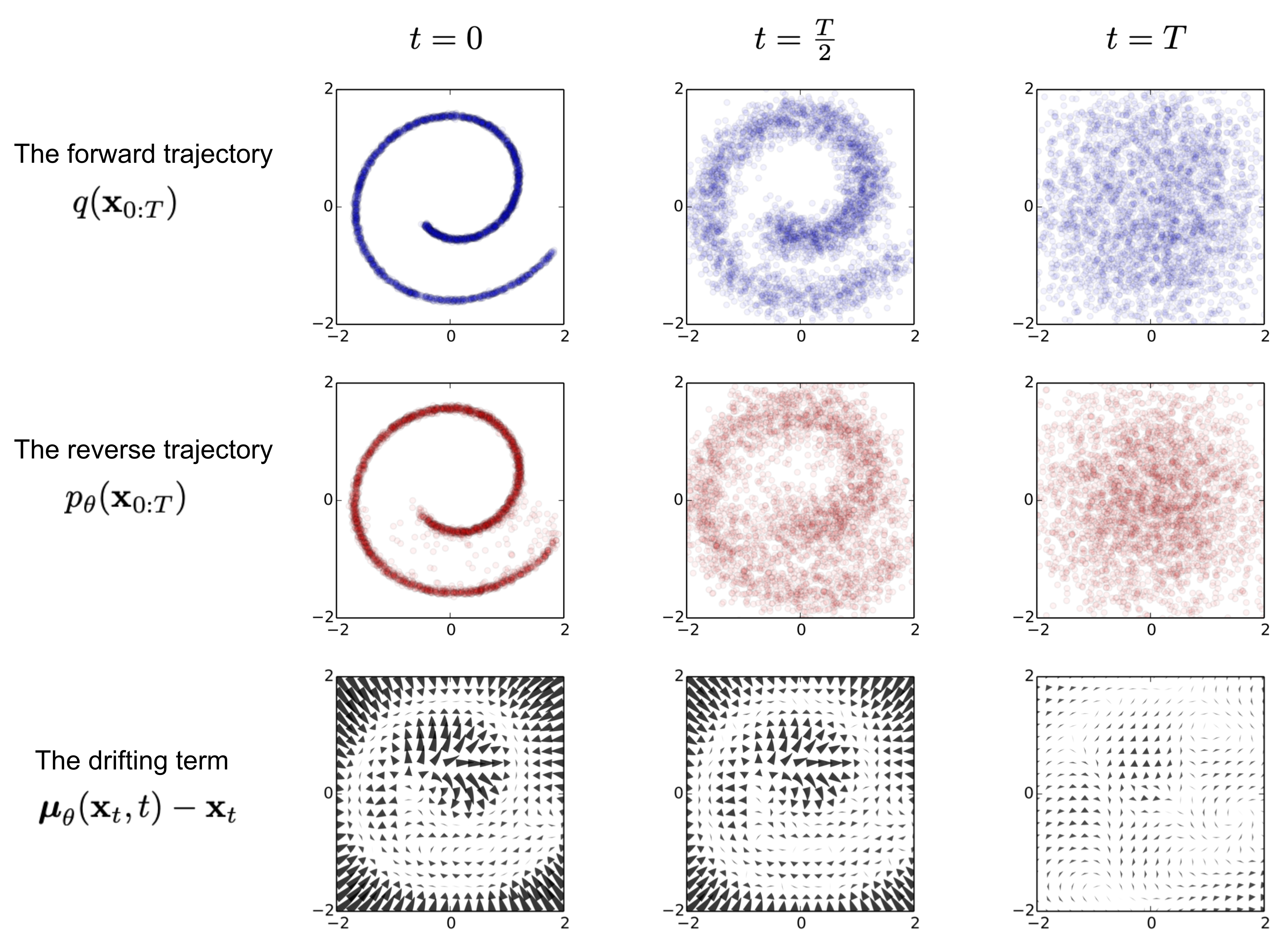
Characteristics of Diffusion Models

Pros:

• Best quality & coverage: diffusion / flow-matching models for images; rapidly improving for video.

Cons:

• High computational cost for training and sampling.

Ultra-compact variant (if space is tight): Diffusion/flow-matching (DiT/RFT) lead in quality; video catching up. Cost = sampling, eased by consistency + distillation.

Generative models overview

Generative models overview

Model	Pros	Cons
VAE	- Explicit likelihood - Fast sampling - Good global structure	- Blurry outputs - Prior bias (Gaussian) - Limited expressiveness
GAN	- Sharp, high-quality images - Fast sampling	- Training instability - Mode collapse - No likelihood
Flow	- Exact likelihood - Invertible - Flexible distributions	- Computationally expensive - Architecture constraints - Difficult to scale
Diffusion	- SOTA quality - Excellent mode coverage - Stable training	- Slow sampling (many steps) - Computationally intensive - Careful tuning required

Each generative model family has distinct tradeoffs. VAEs offer fast training and sampling but produce blurry outputs. GANs generate sharp images but are unstable to train. Flows provide exact likelihoods but are computationally expensive. Diffusion models achieve the best quality but require many sampling steps. Choose based on your application requirements.

JAX Ecosystem

What is JAX?

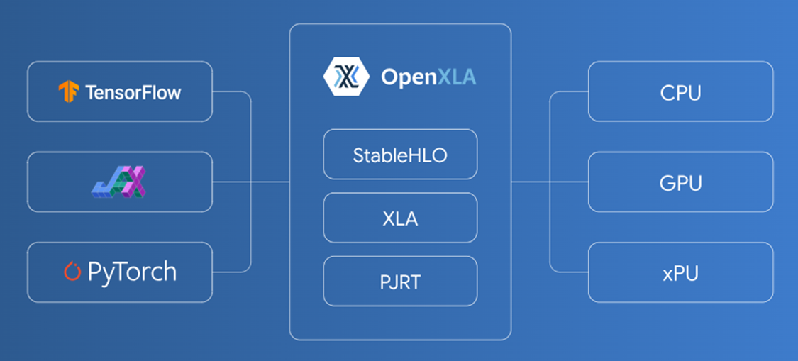
<h2 style="margin:0;">JAX and OpenXLA</h2>

JAX provides a NumPy-compatible API with powerful function transformations. grad computes derivatives, jit compiles to optimized XLA code, vmap vectorizes operations, and pmap parallelizes across devices. JAX enforces functional programming: functions must be pure without side effects. Randomness is explicit via PRNG key splitting. The same code runs efficiently on CPU, GPU, or TPU through XLA compilation.

JAX transforms

JIT (Just in time compilation)

import jax
import jax.numpy as jnp

@jax.jit
def f(x): 
    return jnp.sin(x**2) + jnp.cos(x)

# compiled once, runs fast
y = f(jnp.linspace(0, 3, 1_000))

Auto-vectorization (vmap)

import jax
import jax.numpy as jnp

def score(x, w): 
    return x @ w        # single example

batched_score = jax.vmap(score, in_axes=(0, None))
y = batched_score(X_batch, w)

grad (automatic differentiation)

import jax
import jax.numpy as jnp

def loss(w, x, y):
     return ((x @ w - y)**2).mean()

# grad w.r.t. first arg
dl_dw = jax.grad(loss)(w, x, y)
# 2nd derivative
dl_dl_dw = jax.grad(jax.grad(loss))(w, x, y)
# Hessian matrix
hessian_dw = jax.hessian(loss)(w, x, y)

Multi-device parallelism (shard_map)

import numpy as np
import jax
import jax.numpy as jnp

mesh = jax.sharding.Mesh(np.array(jax.devices()), ('data',))

def double(x):
     return x * 2
     
double_sharded = jax.shard_map(double, mesh=mesh,
        in_specs=jax.sharding.PartitionSpec('data', None),
        out_specs=jax.sharding.PartitionSpec('data', None))

# shard over axis 0
x = jnp.arange(8).reshape(len(jax.devices()), -1) 
y = double_sharded(x)

tiny gradient demo

Computing gradients with PyTorch

import torch
x = torch.randn(10, 5)
w = torch.randn(5, 3, requires_grad=True)

y = x @ w
loss = y.sum()
loss.backward()
print(w.grad)              # gradient lives on tensor state

Computing gradients with JAX

import jax, jax.numpy as jnp

def loss(w, x):
    return (x @ w).sum()

x = jnp.ones((10, 5))
w = jnp.ones((5, 3))
grad_w = jax.grad(loss)(w, x)
print(grad_w)              # returns new array; no hidden state

Implications of functional programming

No impure functions

import jax, jax.numpy as jnp
state = {"counter": 0}

@jax.jit
def bad(x):
    # ❌ side-effect breaks JIT/purity
    state["counter"] += 1
    return x + 1

@jax.jit
def good(x, state):
    # ✅ pure function
    state = {"counter": state["counter"] + 1}  
    return x + 1, state

Explicit PRNG keys

Numpy RNG

import numpy as np
np.random.seed(0)
x = np.random.normal(size=(100,))
y = np.random.uniform(size=(100,))

No inplace mutations

import jax.numpy as jnp
x = jnp.array([1, 2, 3])

@jax.jit
def bad(x):
    x[0] = 10               # ❌ JAX arrays are immutable
    return x

@jax.jit
def good(x):
    x = x.at[0].set(10)     # ✅ returns new array
    return x

JAX RNG

import jax.random as jr
key = jr.PRNGKey(0)
k1 , k2 = jr.split(key)
x = jr.normal(k1, shape=(100,))
y = jr.uniform(k2, shape=(100,))

In general

• All modified variables must be passed explicitly as function arguments and return values.
• All arrays are immutable; use .at[].set() or similar to create modified copies.

Neural nets in JAX (Flax)

Defining a CNN model in PyTorch

import torch.nn as nn
import torch.nn.functional as F

class CNN(nn.Module):
    def __init__(self):
        super().__init__()
        self.c1 = nn.Conv2d(3, 32, 3); self.c2 = nn.Conv2d(32, 64, 3)
        self.fc = nn.Linear(64*6*6, 10)
    def forward(self, x):
        x = F.relu(self.c1(x)); x = F.relu(self.c2(x))
        x = x.view(x.size(0), -1); return self.fc(x)

model = CNN()

Defining a CNN model in Flax

import jax, jax.numpy as jnp
import flax.linen as nn

class CNN(nn.Module):
    @nn.compact
    def __call__(self, x):
        x = nn.relu(nn.Conv(32, (3,3))(x))
        x = nn.relu(nn.Conv(64, (3,3))(x))
        x = x.reshape((x.shape[0], -1))
        return nn.Dense(10)(x)

model = CNN()
params = model.init(jax.random.PRNGKey(0), jnp.ones((1, 3, 8, 8)))

Training step example

One training step in PyTorch

import torch
import torch.nn.functional as F

opt = torch.optim.Adam(model.parameters(), lr=1e-3)

def train_step(x, y):
    opt.zero_grad()
    logits = model(x)
    loss = F.cross_entropy(logits, y)
    loss.backward()
    opt.step()
    return loss.item()

loss = train_step(x_batch, y_batch)

One training step in JAX + Flax + Optax

import jax, jax.numpy as jnp
import optax
from flax.training import train_state

def loss_fn(params, batch):
    logits = model.apply(params, batch["x"])   # forward
    return optax.softmax_cross_entropy_with_integer_labels(
        logits, batch["y"]
    ).mean()

@jax.jit
def train_step(state, batch):
    grads = jax.grad(loss_fn)(state.params, batch)
    return state.apply_gradients(grads=grads)

state = train_state.TrainState.create(
    apply_fn=model.apply,
    params=params,
    tx=optax.adam(1e-3),
)
state = train_step(state, batch)  # one update step

JAX Ecosystem: an overview

FLAX

Neural network library for JAX with modules, layers, optimizers, training loops.

Optax

Gradient processing and optimization library for JAX.

BlackJAX

MCMC sampling library for JAX with HMC, NUTS, SGLD algorithms.

NumPyro

Probabilistic programming library for JAX with Bayesian modeling and inference.

Diffrax

Differential equation solver library for JAX with ODE, SDE, DDE solvers.

Composability + Trade-offs

Strengths

• NumPy-like API; clean function transforms
• Fast & differentiable via XLA + jit
• Powerful composition: jit(vmap(grad(...))), shard_map for multi-device
• Ecosystem: Flax, Optax, BlackJAX, Distrax, Diffrax

Weaknesses

• Steep learning curve (purity, PRNG keys, transformations)
• Fewer off-the-shelf models vs PyTorch
• Some APIs evolving (e.g., sharding tools) → more boilerplate at first

Hands-On: Cosmology Applications

GZ10 Dataset

Galaxy Zoo 10 from MultimodalUniverse:

from datasets import load_dataset
ds = load_dataset("MultimodalUniverse/gz10")

Dataset statistics:

• ~17,700 galaxy images
• RGB images (256×256 pixels)
• Fields: gz10_label, redshift, object_id

For this workshop: Downsize to 32×32 or 64×64 for

Explore the dataset

Notebook link : Generative_AI_JAX_GZ10_VAE.ipynb

Example A: Variational Autoencoder for galaxies

Variational Autoencoder

Train a VAE on GZ10 galaxies and analyze latent space

Notebook link : Generative_AI_JAX_GZ10_VAE.ipynb

Example B : Using a classifier from the latent space

VAE latent space to redshift

Classify galaxy morphology from VAE latent space

Notebook link : Generative_AI_JAX_GZ10_VAE_Classifier.ipynb