Bayesian Inference for Cosmology with JAX
2025-05-01


Inference in Cosmology: The Frequentist Pipeline


- cosmological parameters (Ω): matter density, dark energy, etc.
- Predict observables: CMB, galaxies, lensing
- Extract summary statistics: \(P(k)\), \(C_\ell\) , 2PCF
- Compute likelihood: \(L(\Omega \vert data)\)
- Estimate \(\hat{\Omega}\) via maximization (\(\chi^2\) fitting)
Frequentist Toolbox
- Optimizers/Gradient descent
- 2-point correlation function (2PCF)
- Power spectrum fitting: \(P(k)\), \(C_\ell\)
Inference in Cosmology: The Bayesian Pipeline


- Start from summary statistics: \(P(k)\), \(C_\ell\) , 2PCF
- Sample from a Prior \(P(\Omega)\)
- Compute likelihood: \(L(Obs \vert \Omega)\)
- Sampler from the Posterior \(P(\Omega \vert Obs)\)
Bayesian Toolbox
- Priors encode beliefs: \(P(\Omega)\)
- Hierarchical Bayesian Modeling (HBM)
- Probabilistic programming (e.g., NumPyro)
- Gradient-based samplers: HMC, NUTS
Inference in Cosmology: The Bayesian Pipeline

- Prior: Theory-driven assumptions \(P(\Omega)\)
- Latent variables: Hidden/unobserved \(z \sim P(z \mid \Omega)\)
- Likelihood: Generates observables \(P(\text{Obs} \mid \Omega, z)\)
- Posterior: infer \(P(\Omega \mid \text{Obs})\)
Inference in Cosmology: The Bayesian Pipeline
Bayes’ Rule with all components:
Full decomposition of the posterior. The denominator marginalizes over all possible parameters.
\[ \underbrace{P(\Omega \mid \text{Obs})}_{\text{Posterior}} = \frac{ \underbrace{P(\text{Obs} \mid \Omega)}_{\text{Likelihood}} \cdot \underbrace{P(\Omega)}_{\text{Prior}} }{ \underbrace{ \int P(\text{Obs} \mid \Omega) P(\Omega) \, d\Omega }_{\text{Evidence}} } \]
\[ \underbrace{P(\Omega \mid \text{Obs})}_{\text{Posterior}} = \frac{ \underbrace{\int P(\text{Obs} \mid \Omega, z)\, P(z \mid \Omega)\, dz}_{\text{Likelihood (marginalized over latent $z$)}} \cdot \underbrace{P(\Omega)}_{\text{Prior}} }{ \underbrace{ \int \left[ \int P(\text{Obs} \mid \Omega, z)\, P(z \mid \Omega)\, dz \right] P(\Omega)\, d\Omega }_{\text{Evidence}} } \]
In practice, we drop the evidence term when sampling — it’s a constant.
\[ P(\Omega \mid \text{Obs}) \propto \underbrace{\int P(\text{Obs} \mid \Omega, z)\, P(z \mid \Omega) \, dz}_{\text{Marginal Likelihood}} \cdot \underbrace{P(\Omega)}_{\text{Prior}} \]
\[ \log P(\Omega \mid \text{Obs}) = \log P(\text{Obs} \mid \Omega) + \log P(\Omega) \]
Bayes’ Rule in Practice
The posterior combines theory (prior) and data (likelihood) to infer cosmological parameters.
Latent variables \(z\) encode hidden structure (e.g., initial fields, nuisance parameters).
The evidence is often ignored during sampling (it’s constant).
Model comparison via the Bayes Factor:
\[ \text{Bayes Factor} = \frac{P(\text{Obs} \mid \mathcal{M}_1)}{P(\text{Obs} \mid \mathcal{M}_2)} \]
Two Roads to Inference: Frequentist and Bayesian
Conceptual Differences
| Concept | Frequentist | Bayesian |
|---|---|---|
| Parameters | Fixed but unknown | Random variables with a prior |
| Goal | Point estimate (e.g. MLE) | Full distribution (posterior over parameters) |
| Uncertainty | From data variability | From parameter uncertainty (posterior) |
| Prior Knowledge | Not used | Explicitly included via prior \(P(\Omega)\) |
| Interval Meaning | Confidence interval: “95% of experiments contain truth” | Credible interval: “95% chance truth is in this range” |
| Likelihood Role | Central in \(\chi^2\) minimization, fits | Combined with prior to form posterior |
| Inference Output | Best-fit estimate + error bars | Posterior distribution |
| Tooling | Optimization (e.g. χ², maximum likelihood) | Sampling (e.g. MCMC, HMC, NUTS) |
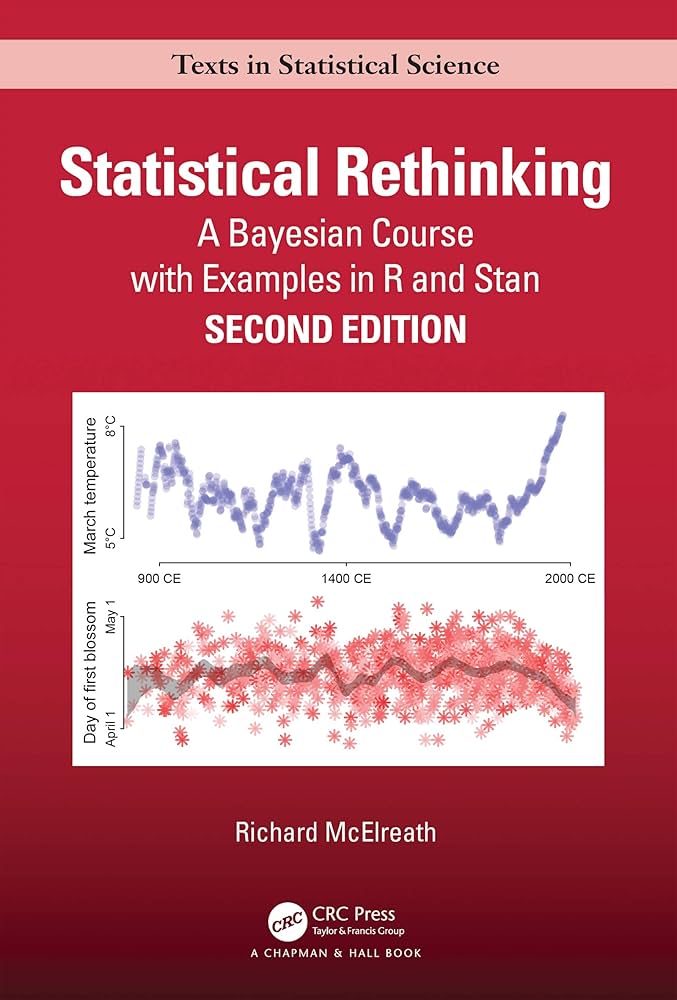
Although these approaches are often contrasted, they’re not mutually exclusive. Modern workflows — like causal inference in Statistical Rethinking — draw on both perspectives. Bayesian methods offer a formal way to combine theory and data, especially powerful when simulations are involved.
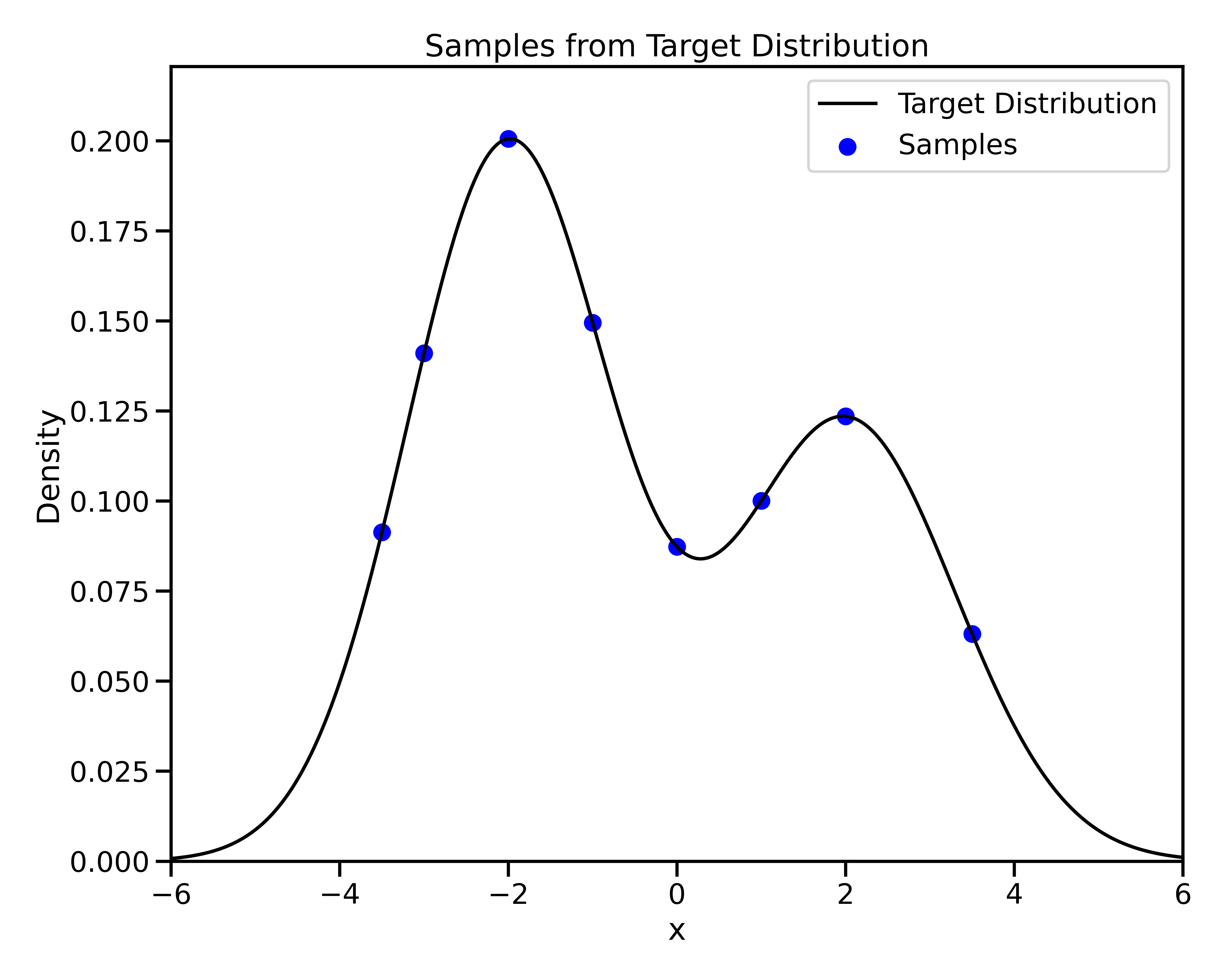
Sampling the Posterior: The Core Loop

The Sampling Loop:
- Start from a sample \((\Omega^t, z^t)\)
- Propose new sample \((\Omega', z')\)
- Compute acceptance probability
- Accept or reject proposal
- Repeat and store accepted samples ⟶ posterior
Goal: Explore the full shape of the posterior
(even in high-dim, non-Gaussian spaces)
Key Takeaways
- Most samplers follow this accept/reject loop
- Differ by how they propose samples: – Random walk (e.g., MH) – Gradient-guided (e.g., HMC, NUTS)
- Some skip rejection (e.g., Langevin, VI)
Sampling Algorithms at a Glance
Metropolis-Hastings (MCMC)
Propose: Random walk \(\Omega' \sim \mathcal{N}(\Omega^t, \sigma^2)\)
Accept:
\[ \alpha = \min\left(1, \frac{P(\text{Obs} \mid \Omega') P(\Omega')}{P(\text{Obs} \mid \Omega^t) P(\Omega^t)}\right) \]
Hamiltonian Monte Carlo (HMC)
- Propose: Simulate physics Trajectory via gradients \(\nabla\_\Omega \log P(\text{Obs} \mid \Omega)\)
- Accept: Based on Hamiltonian energy conservation. \(\alpha = \min(1, e^{\mathcal{H}(\Omega^t, p^t) - \mathcal{H}(\Omega', p')})\)
NUTS (No-U-Turn Sampler) Same as HMC, but auto-tunes:
- Step size
- Trajectory length (stops before looping back)
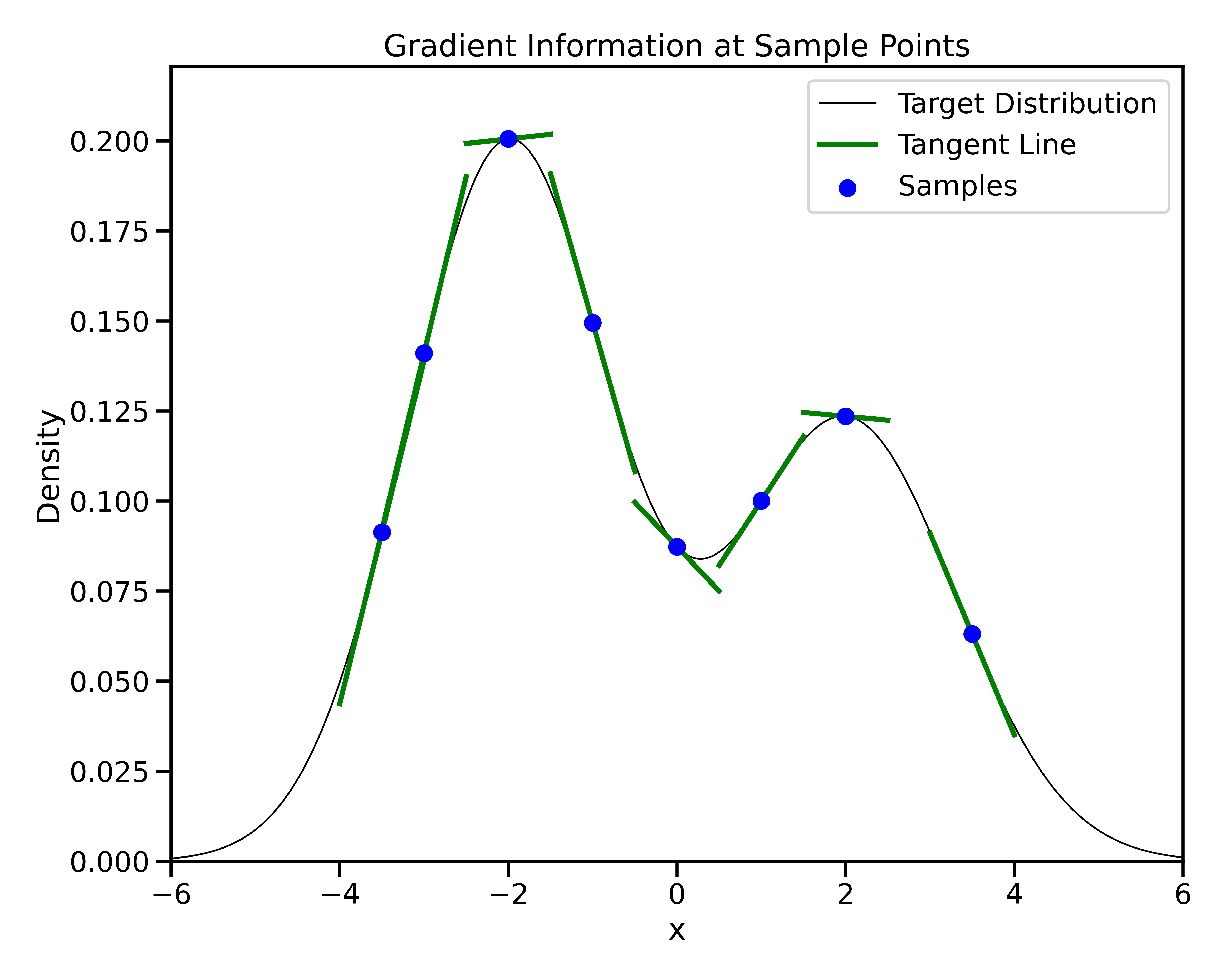
Gradient-Based Sampling in Action
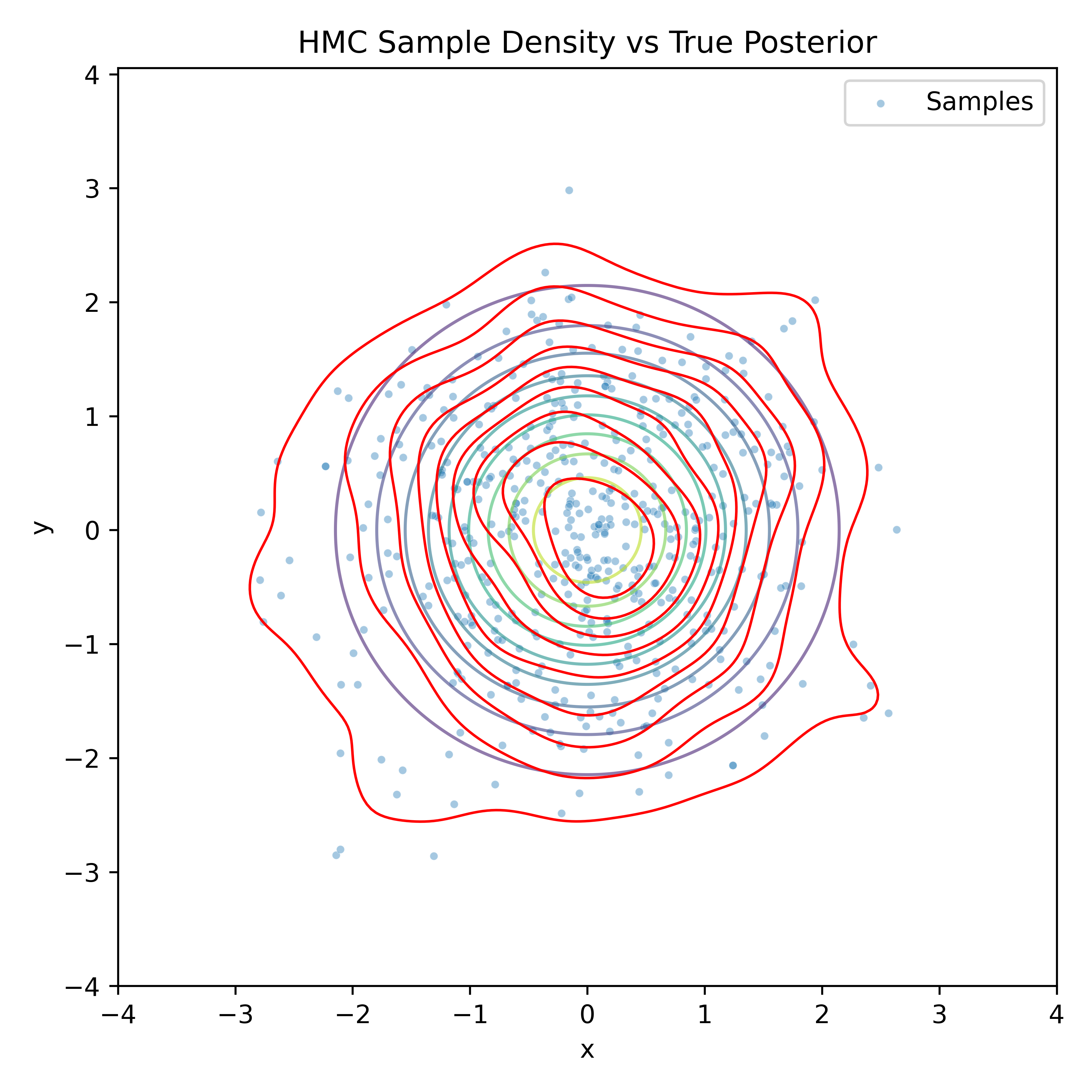
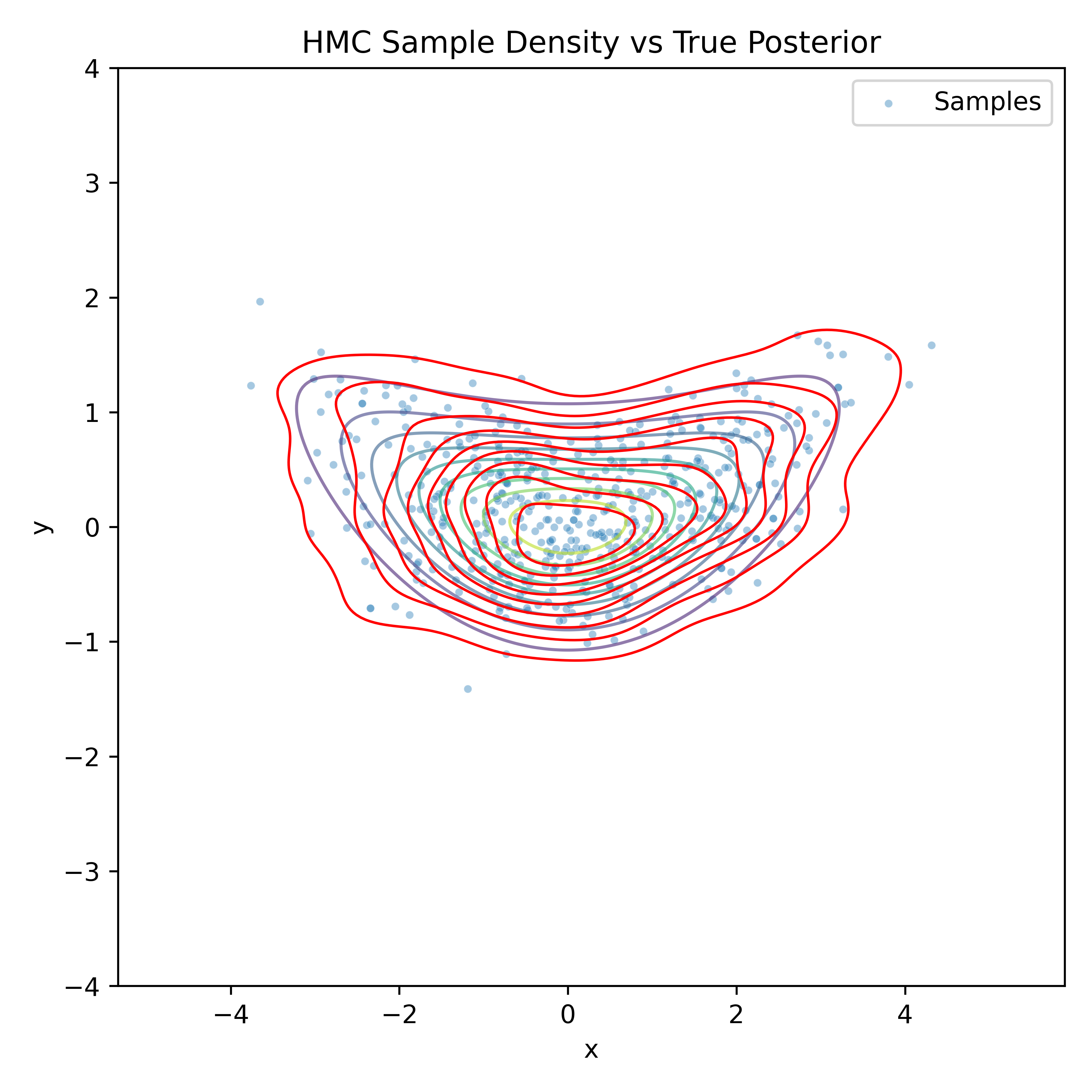

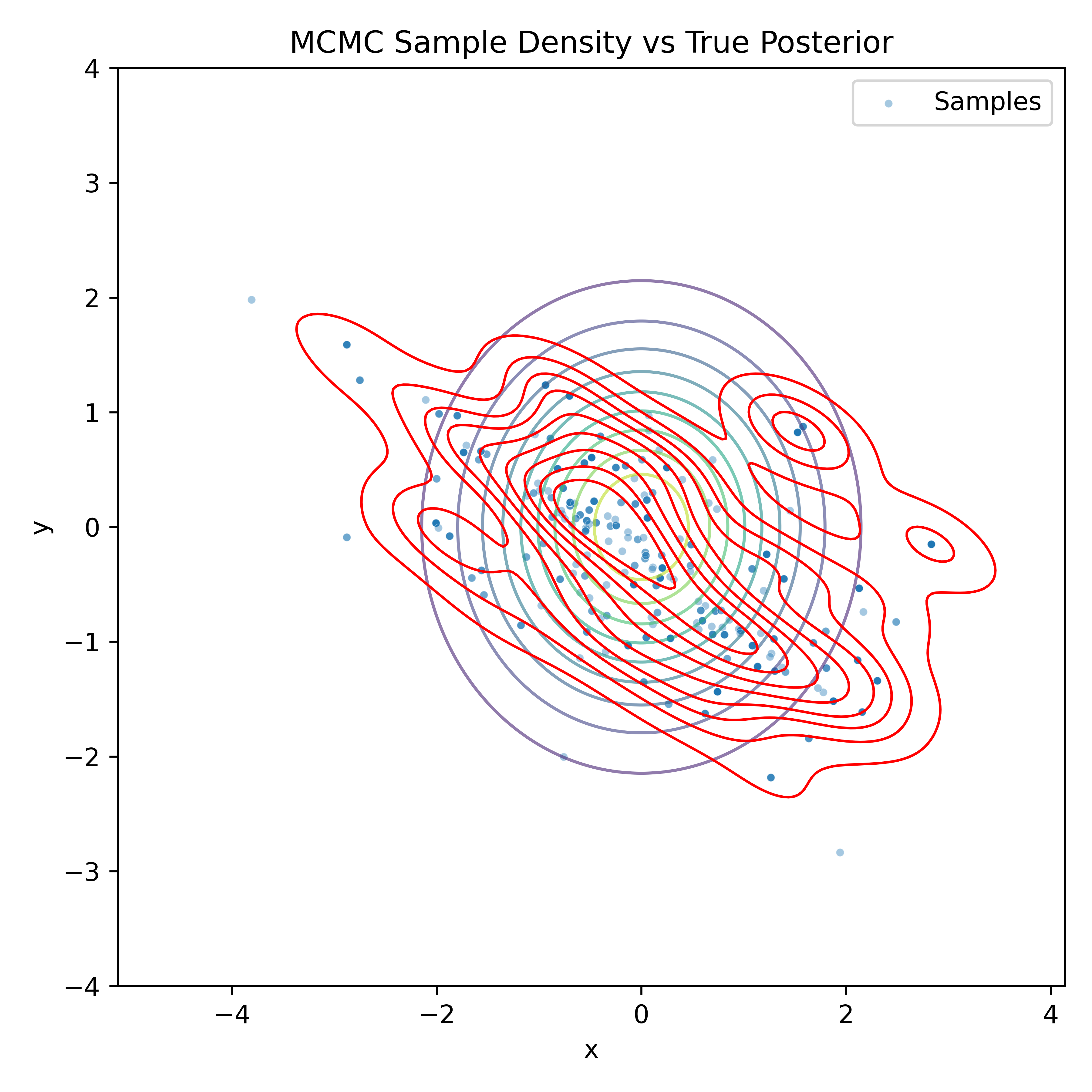

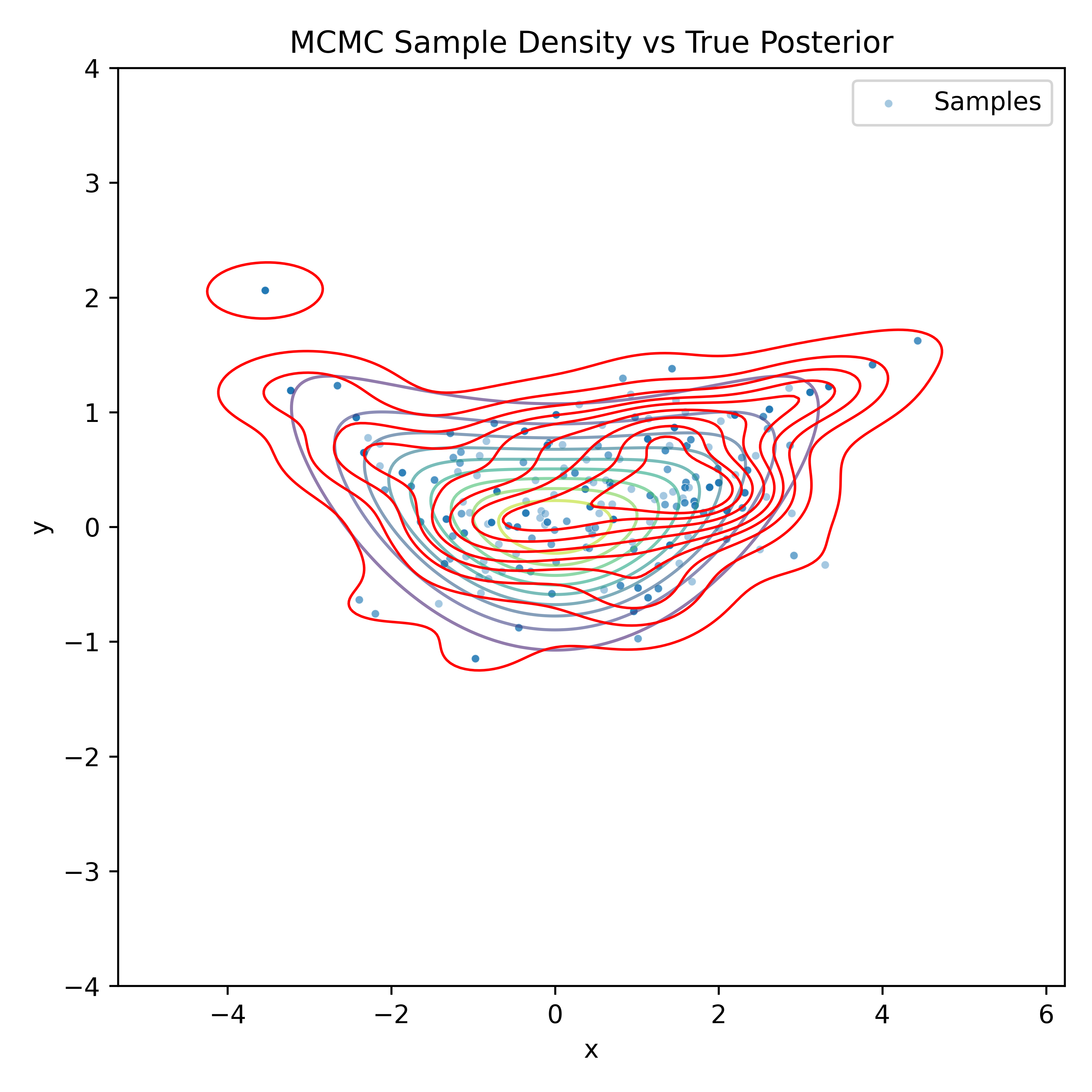
Gradient-Based Sampling in Action
- In high dimensions, random walk proposals (MCMC) often land in low-probability regions ⟶ low acceptance.
- To maintain acceptance, step size must shrink like \(1/\sqrt{d}\) ⟶ very slow exploration.
- HMC uses gradients to follow high-probability paths ⟶ better samples, fewer steps.
Differentiable Inference with JAX
When it comes to gradients, always think of JAX.
An Easy pythonic API
Easily accessible gradients using GRAD
A Recipe for Bayesian Inference
1. Probabilistic Programming Language (PPL) NumPyro:
2. Computing Likelihoods JAX-Cosmo:
3. Sampling the Posterior NumPyro & Blackjax:


Full Field Inference with Forward Models
Bayesian Inference using power spectrum data:
Bayesian Inference using full field data:


- Recap: Bayesian inference maps theory + data → posterior
- Cosmological Forward models
- Start from cosmological + latent parameters
- Sample initial conditions
- Evolve using N-body simulations
- Predict convergence maps in tomographic bins
- Simulation-Based Inference
- Compare predictions to real survey maps
- Build a likelihood from the forward model
- Infer cosmological parameters from full field data
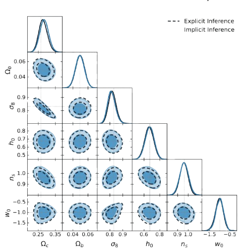
Full Field vs. Summary Statistics
- Preserves non-Gaussian structure lost in summaries
- Enables tighter constraints in nonlinear regimes
- Especially useful in high-dimensional inference problems
- See: Zeghal et al. (2024), Leclercq et al. (2021)
- 🔜 a talk on this topic this Thursday