JAXPM: A JAX-Based Framework for Scalable and Differentiable Particle Mesh Simulations

Wassim Kabalan

Alexandre Boucaud, François Lanusse

2025-05-01

Outline for This Presentation

• Beyond Summary Statistics Inference in Cosmology
  
  
• Building N-body Simulators for Cosmological Inference
  
  
• Modeling Observables: Weak Lensing & Lightcones
  
  
• Scaling Up: Distributed, Differentiable Simulations

The Traditional Approach to Cosmological Inference

• cosmological parameters (Ω): matter density, dark energy, etc.
• Predict observables: CMB, galaxies, lensing
• Extract summary statistics: \(P(k)\), \(C_\ell\) , 2PCF
• Compute likelihood: \(L(\Omega \vert data)\)
• Estimate \(\hat{\Omega}\) via maximization (\(\chi^2\) fitting)

Summary Statistics Based Inference

• Traditional inference uses summary statistics to compress data.
• Power spectrum fitting: \(P(k)\), \(C_\ell\)
• It misses complex, non-linear structure in the data

“Most of modern cosmological inference pipelines rely on summary statistics — things like the power spectrum P(k)P(k) or angular power spectrum CℓCℓ​.”

“These work well under the assumption that most of the information is encoded in second-order statistics — basically, the correlations between pairs of points.”

“But this approach ignores all the higher-order structure — the full non-linear complexity that emerges in the formation of cosmic structure.”

Even higher-order statistics (like bispectrum or 3-point correlations) still reduce the data, and fail to capture the entire structure or allow for fully Bayesian inference over the field.

“And that’s the motivation for moving beyond summary statistics…”

The Traditional Approach to Cosmological Inference

Credit: Natalia Porqueres

Jeffrey et al. (2024)

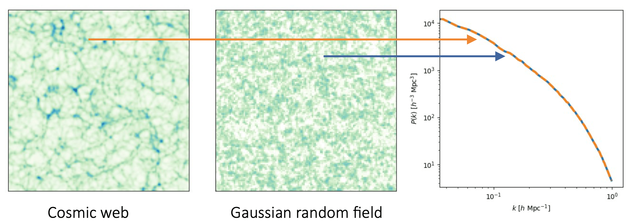
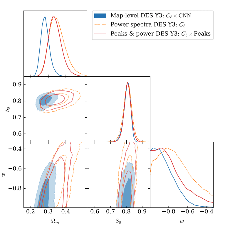
• Summary statistics (e.g. P(k)) discard the non-Gaussian features.
• Gradient-based curve fitting does not recover the true posterior shape.

How to maximize the information gain?

From Summary Statistics to Likelihood Free Inference

Bayes’ Theorem

\[ p(\theta \mid x_0) \propto p(x_0 \mid \theta) \cdot p(\theta) \]

• Prior: Encodes our assumptions about parameters \(\theta\)
• Likelihood: How likely the data \(x_0\) is given \(\theta\)
• Posterior: What we want to learn — how data updates our belief about \(\theta\)

• Simulators become the bridge between cosmological parameters and observables.
• How to use simulators allow us to go beyond summary statistics?

From Summary Statistics to Likelihood Free Inference

Implicit Inference

• Treats the simulator as a black box — we only require the ability to simulate \((\theta, x)\) pairs.

• No need for an explicit likelihood — instead, use simulation-based inference (SBI) techniques

• Often relies on compression to summary statistics \(t = f_\phi(x)\), then approximates \(p(\theta \mid t)\).

Explicit Inference

• Requires a differentiable forward model or simulator.

• Treat the simulator as a probabilistic model and perform inference over the joint posterior \(p(x \mid \theta, z)\)

• Computationally demanding — but provides exact control over the statistical model.

Implicit Inference

Explicit Inference

Implicit inference

Simulation-Based Inference Loop

• Sample parameters \(\theta_i \sim p(\theta)\)
• Run simulator \(x_i = p(x \vert \theta_i)\)
• Compress observables \(t_i = f_\phi(x_i)\)
• Train a density estimator \(\hat{p}_\Phi(\theta \mid f_\phi(x))\)

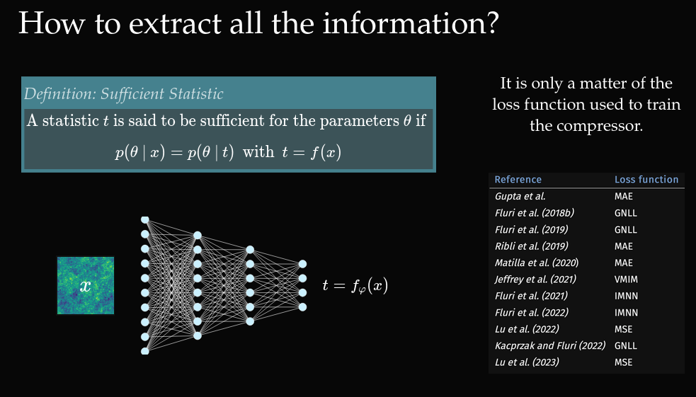
• Neural Summarisation (Zeghal & Lanzieri et al 2025).
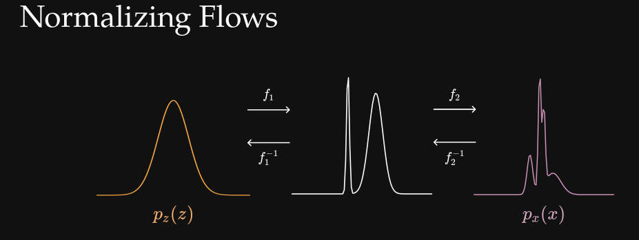
• Normalizing Flows (Zeghal et al. 2022).
• ✅ Works with non-differentiable or stochastic simulators
• ❌ Requires an optimal compression function \(f_\phi\)

Explicit inference

The goal is to reconstruct the entire latent structure of the Universe — not just compress it into summary statistics. To do this, we jointly infer:

\[ p(\theta, z \mid x) \propto p(x \mid \theta, z) \, p(z \mid \theta) \, p(\theta) \]

Where:

• \(\theta\): cosmological parameters (e.g. matter density, dark energy, etc.)

• \(z\): latent fields (e.g. initial conditions of the density field)

• \(x\): observed data (e.g. convergence maps or galaxy fields)

The challenge of explicit inference

• The latent variables \(z\) typically live in very high-dimensional spaces — with millions of degrees of freedom.

• Sampling in this space is intractable using traditional inference techniques.

• We need samplers that can scale efficiently to high-dimensional latent spaces and Exploit gradients from differentiable simulators
• This makes differentiable simulators essential for modern cosmological inference.
• Particle Mesh (PM) simulations offer a scalable and differentiable solution.

Explicit Inference

Particle Mesh Simulations

Compute Forces via PM method

• Start with particles \(\mathbf{x}_i, \mathbf{p}_i\)
  
• Interpolate to mesh: \(\rho(\mathbf{x})\)
  
• Solve Poisson’s Equation: \[ \nabla^2 \phi = -4\pi G \rho \]
• In Fourier space: \[ \mathbf{f}(\mathbf{k}) = i\mathbf{k}k^{-2}\rho(\mathbf{k}) \]

Time Evolution via ODE

• PM uses Kick-Drift-Kick (symplectic) scheme:
  • Drift: \(\mathbf{x} \leftarrow \mathbf{x} + \Delta a \cdot \mathbf{v}\)
  • Kick: \(\mathbf{v} \leftarrow \mathbf{v} + \Delta a \cdot \nabla \phi\)

• Fast and scalable approximation to gravity.
• A cycle of FFTs and interpolations.
• Sacrifices small-scale accuracy for speed and differentiability.
• Current implementations JAXPM v0.1, PMWD and BORG.

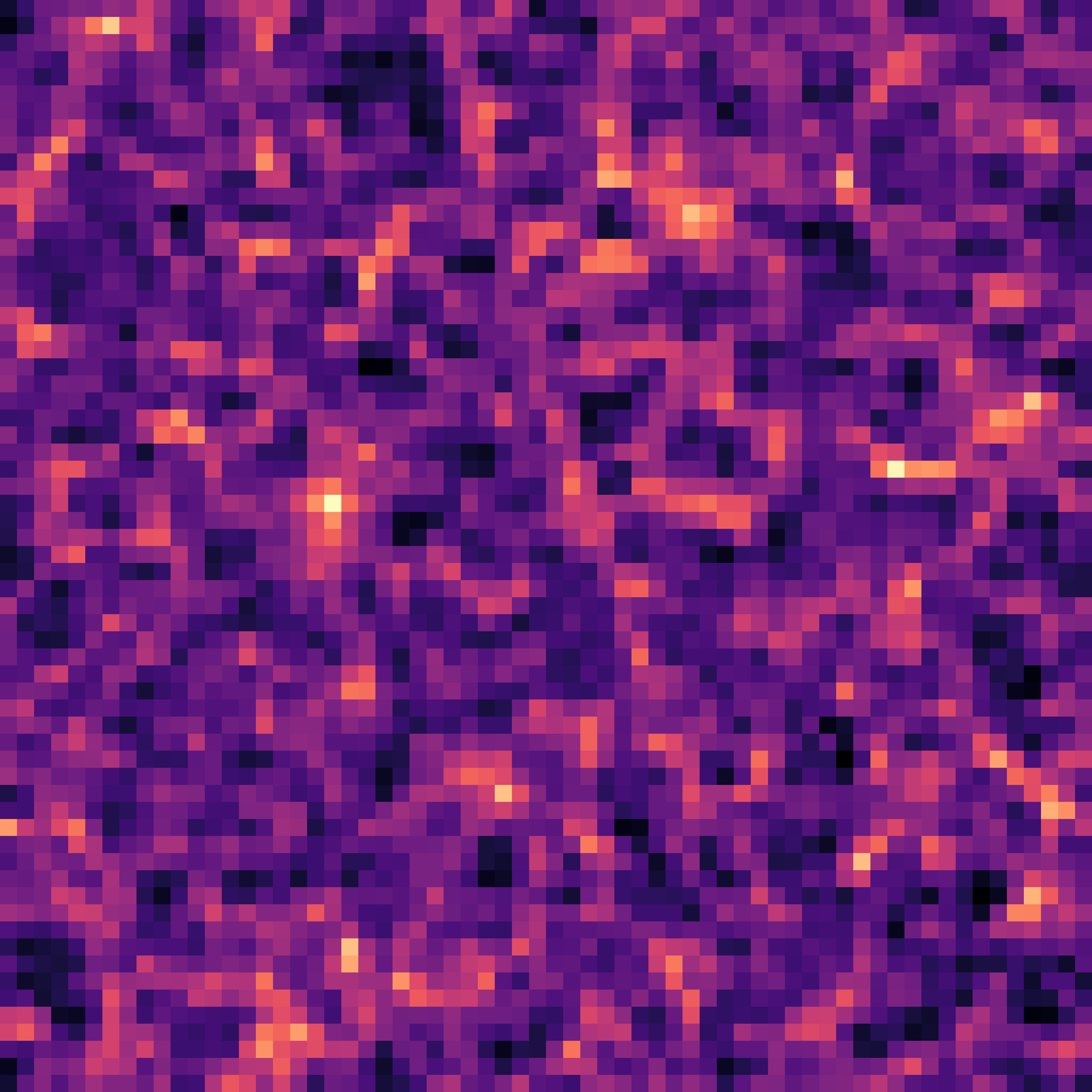
Using Full-Field Inference with Weak Lensing

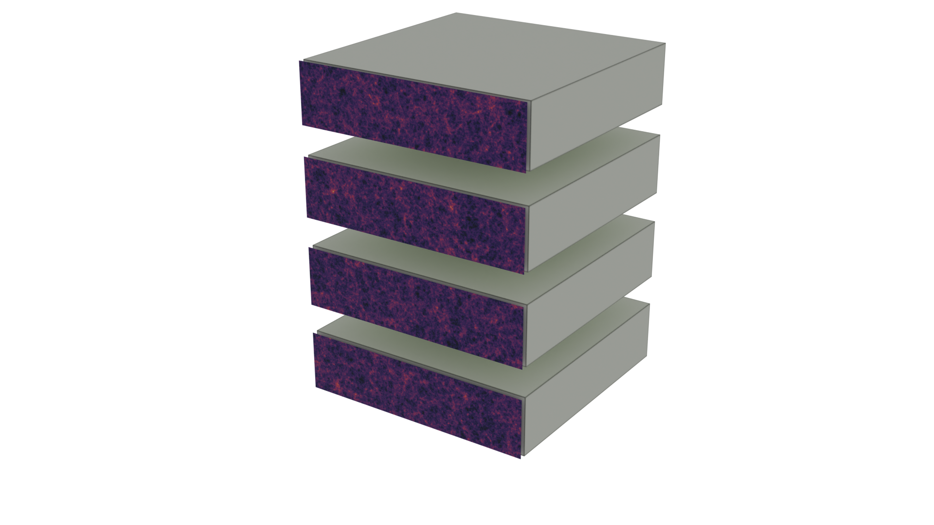
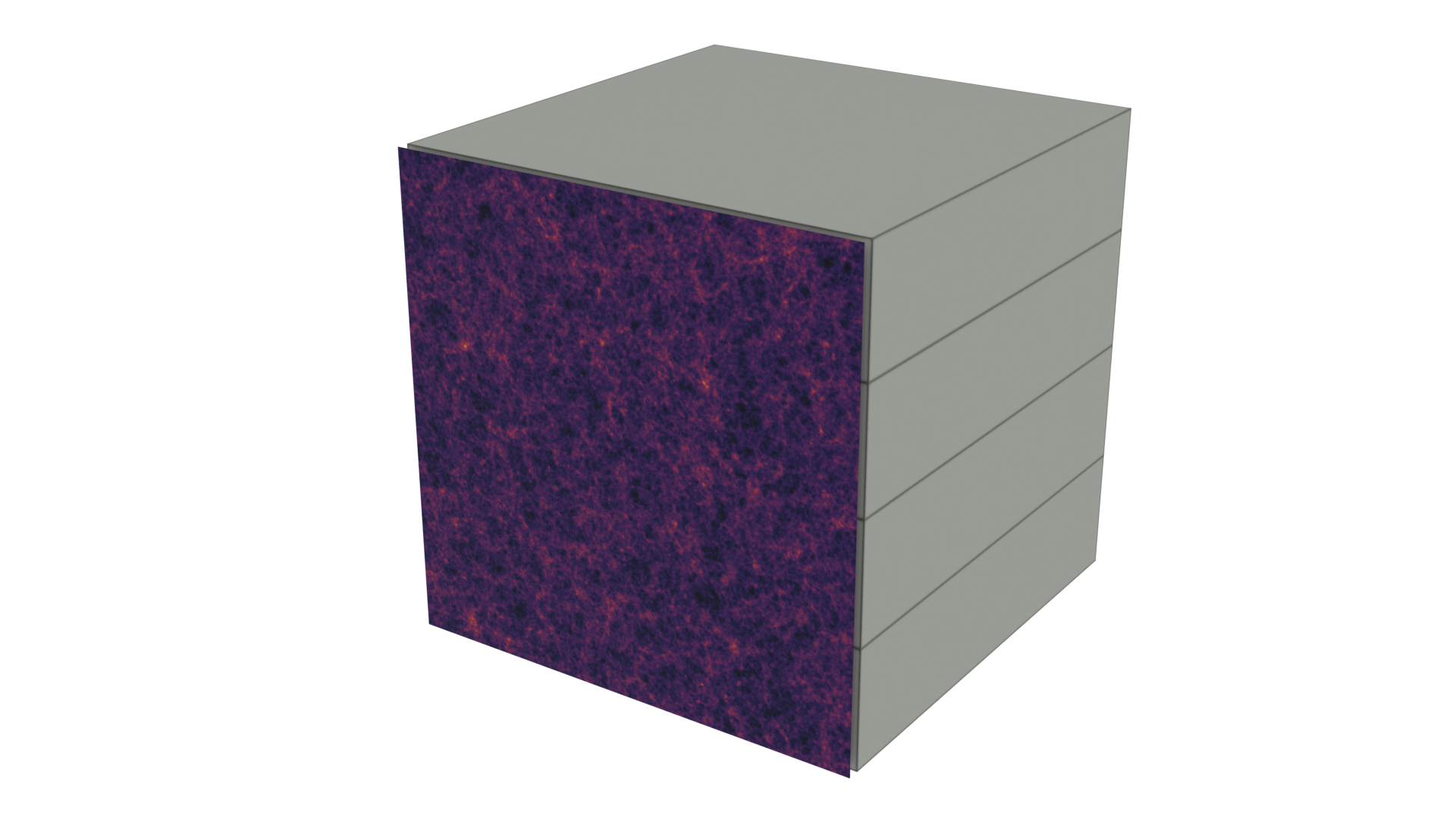
From 3D Structure to Lensing Observables

• Simulate structure formation over time, taking snapshots at key redshifts
• Stitch these snapshots into a lightcone, mimicking the observer’s view of the universe
• Combine contributions from all slabs to form convergence maps
• Use the Born approximation to simplify the lensing calculation

Born Approximation for Convergence

\[ \kappa(\boldsymbol{\theta}) = \int_0^{r_s} dr \, W(r, r_s) \, \delta(\boldsymbol{\theta}, r) \]

Where the lensing weight is:

\[ W(r, r_s) = \frac{3}{2} \, \Omega_m \, \left( \frac{H_0}{c} \right)^2 \, \frac{r}{a(r)} \left(1 - \frac{r}{r_s} \right) \]

Can we start doing inference?

“So we’ve built a forward model — from cosmology to lensing maps. Now comes the big question: can we start doing inference?” (click)

The impact of resolution on simulation accuracy

\(512^3\) Resolution mesh

\(256^3\) Resolution mesh

\(64^3\) Resolution mesh

-

Biased Posterior

“Well… not yet. Not if we care about accuracy.” “Here’s what happens as we vary the resolution of the simulation mesh. Visually, the structure starts to break down. But more importantly, we lose power on small scales — and that directly biases the inferred cosmological parameters.” “So even if our inference machinery is technically running — the science is wrong.” “Low-resolution simulations introduce a significant systematic bias in the inferred parameters — even if the rest of the pipeline is perfect.”

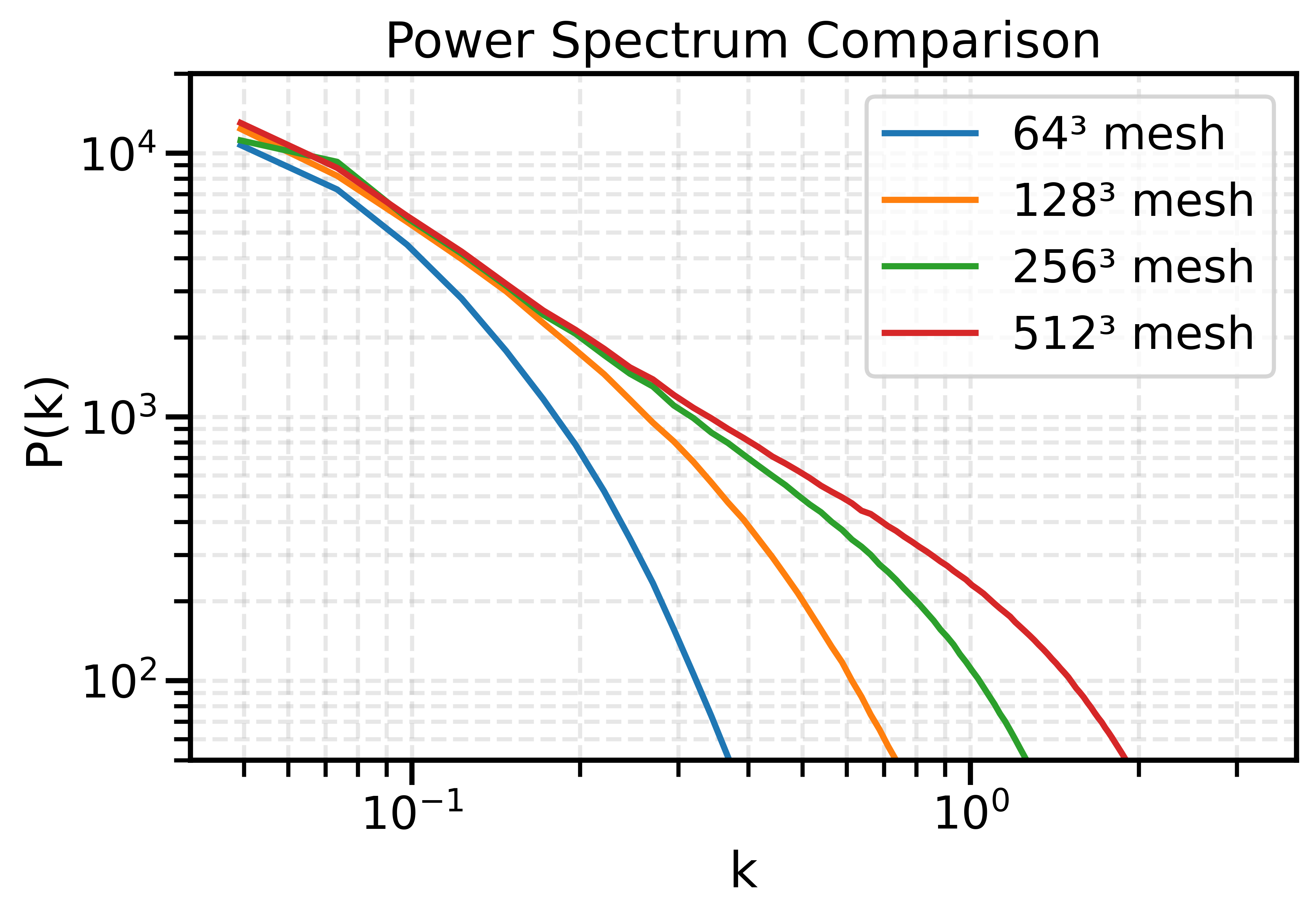
When the Simulator Fails, the Model Fails

Inference is only as good as the simulator it depends on.

• If we want to model complex phenomena like galaxy painting, baryonic feedback, or non-linear structure formation, our simulator must be not only fast, but also physically accurate.
• A decent resolution for weak lensing requires about 1 grid cell per Mpc/h — both for angular resolution and structure fidelity.

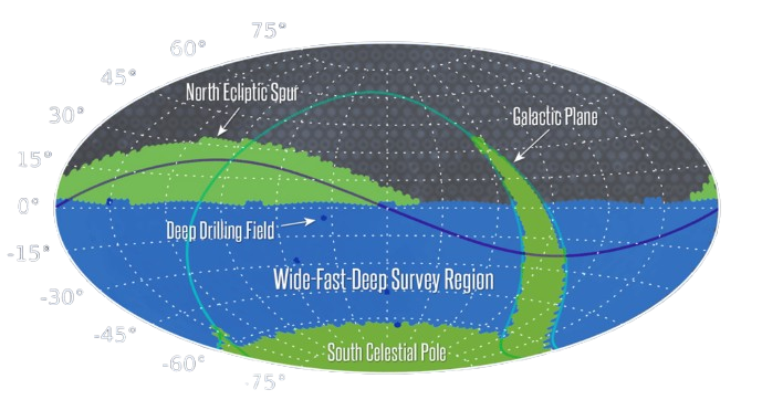
Scaling Up the simulation volume: The LSST Challenge

LSST Scan Range

• Covers ~18,000 deg² (~44% of the sky)
• Redshift reach: up to z ≈ 3
• Arcminute-scale resolution
• Requires simulations spanning thousands of Mpc in depth and width

LSST Survey Footprint

• Simulating even a (1 Gpc/h)³ subvolume at 1024³ mesh resolution requires:
  • ~54 GB of memory for a simulation with a single snapshot
  • Gradient-based inference and multi-step evolution push that beyond 100–200 GB

Takeaway

• LSST-scale cosmological inference demands multiple (Gpc/h)³ simulations at high resolution.
  Modern high-end GPUs cap at ~80 GB, so even a single box requires multi-GPU distributed simulation — both for memory and compute scalability.

Jean Zay HPC - IDRIS

We Need Scalable Distributed Simulations

Distributed Particle Mesh Simulation

Particle Mesh Simulation

Particle Mesh Simulation

Particle Mesh Simulation

Force Computation is Easy to Parallelize

• Poisson’s equation in Fourier space:
  \[ \nabla^2 \phi = -4\pi G \rho \]

• Gravitational force in Fourier space:
  \[ \mathbf{f}(\mathbf{k}) = i\mathbf{k}k^{-2}\rho(\mathbf{k}) \]

• Each Fourier mode \(\mathbf{k}\) can be computed independently using JAX
  

• Perfect for large-scale, parallel GPU execution

Fourier Transform requires global communication

jaxDecomp: Distributed 3D FFT and Halo Exchange

• Distributed 3D FFT using domain decomposition
  
• Fully differentiable, runs on multi-GPU and multi-node setups
  
• Designed as a drop-in replacement for jax.numpy.fft.fftn
  
• Open source and available on PyPI \(\Rightarrow\) pip install jaxdecomp
• Halo exchange for mass conservation across subdomains

FFT

Halo Exchange

Distributed Particle Mesh Simulation

Particle Mesh Simulation

Cloud In Cell (CIC) Interpolation

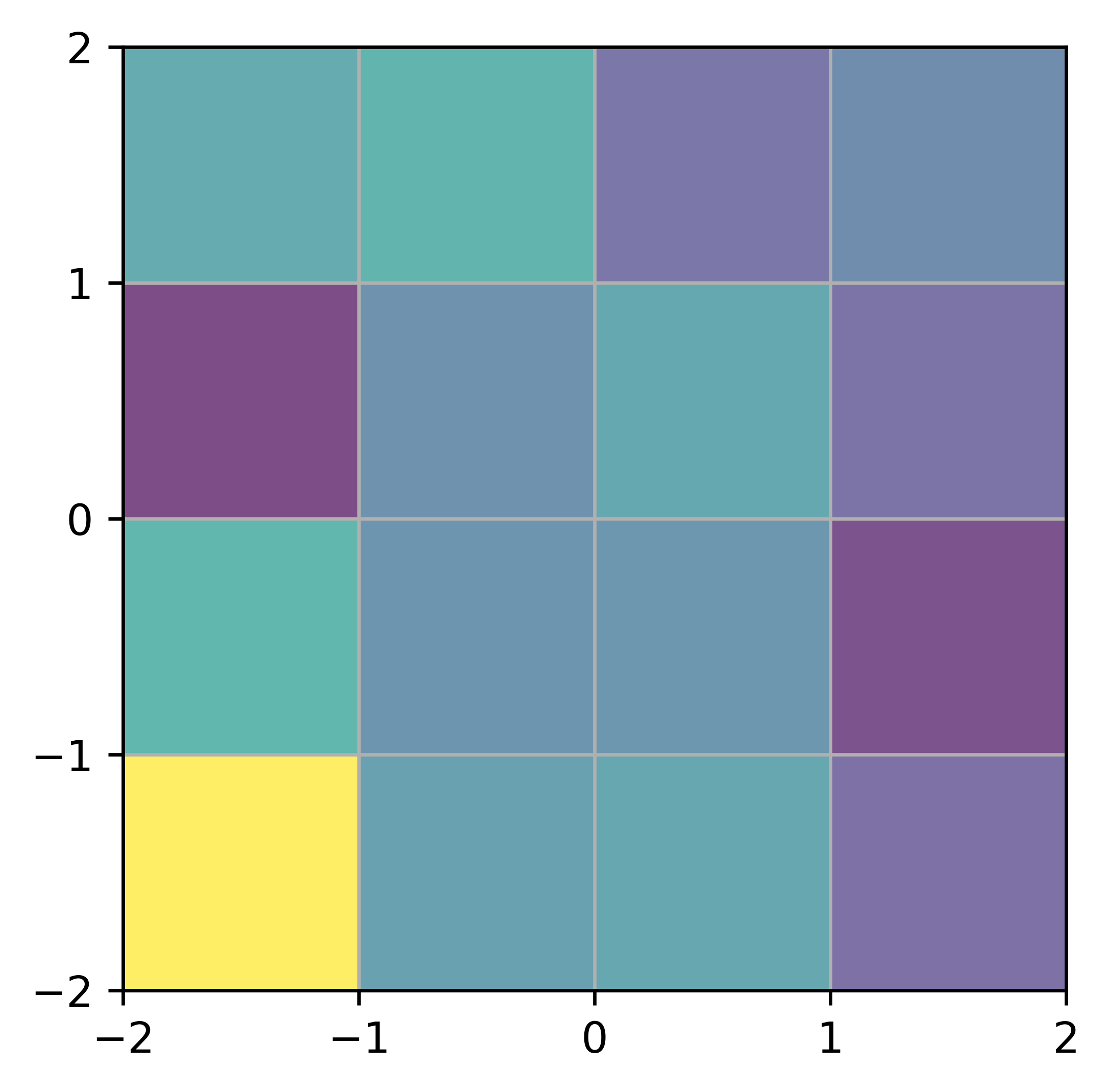
Mass Assignment and Readout

The Cloud-In-Cell (CIC) scheme spreads particle mass to nearby grid points using a linear kernel:

• Paint to Grid (mass deposition): \[ g(\mathbf{j}) = \sum_i m_i \prod_{d=1}^{D} \left(1 - \left|p_i^d - j_d\right|\right) \]

• Read from Grid (force interpolation): \[ v_i = \sum_{\mathbf{j}} g(\mathbf{j}) \prod_{d=1}^{D} \left(1 - \left|p_i^d - j_d\right|\right) \]

Distributed Cloud In Cell (CIC) Interpolation

• In distributed simulations, each subdomain handles a portion of the global domain

• Boundary conditions are crucial to ensure physical continuity across subdomain edges

• CIC interpolation assigns and reads mass from nearby grid cells — potentially crossing subdomain boundaries

• To avoid discontinuities or mass loss, we apply halo exchange:

  • Subdomains share overlapping edge data with neighbors
  • Ensures correct mass assignment and gradient flow across boundaries

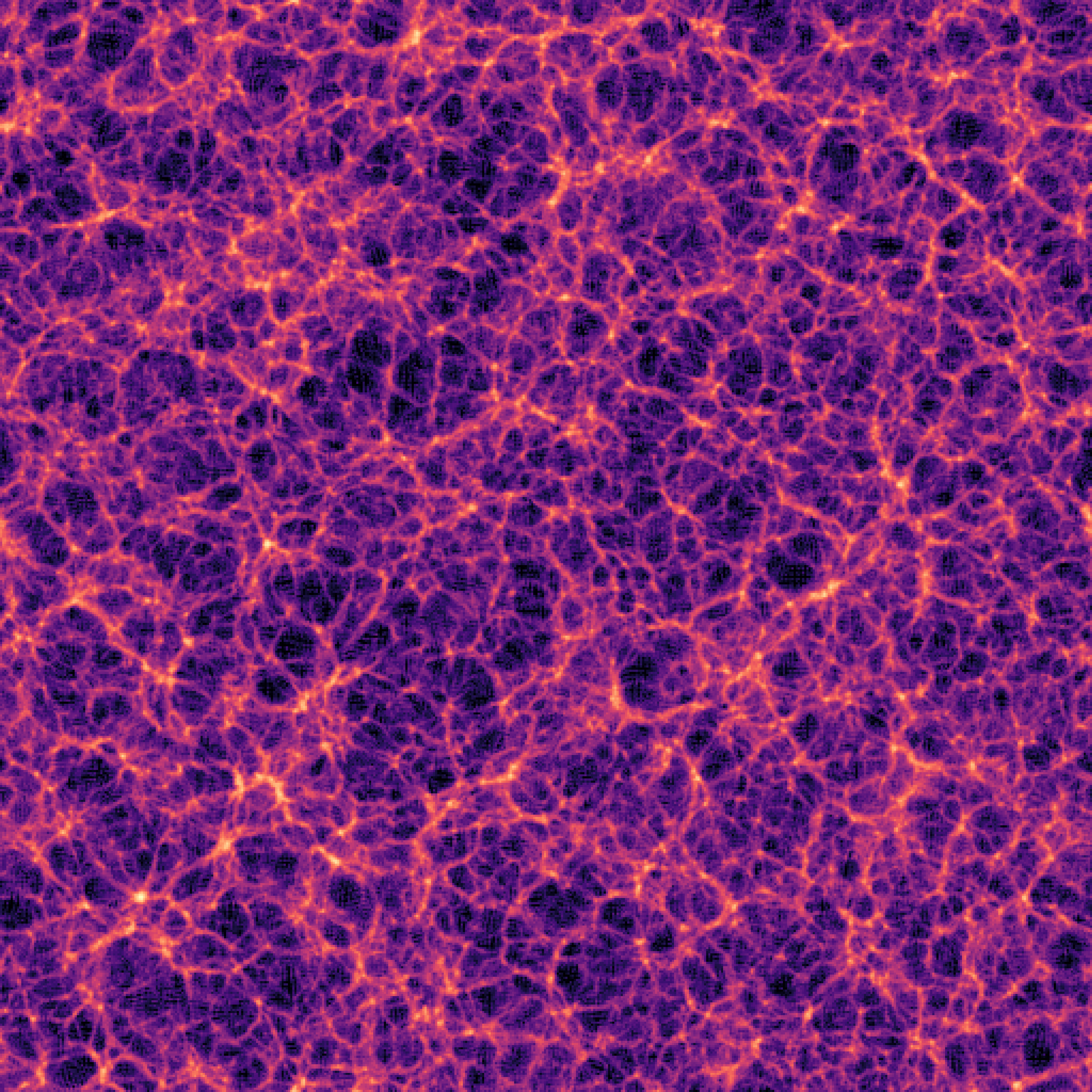
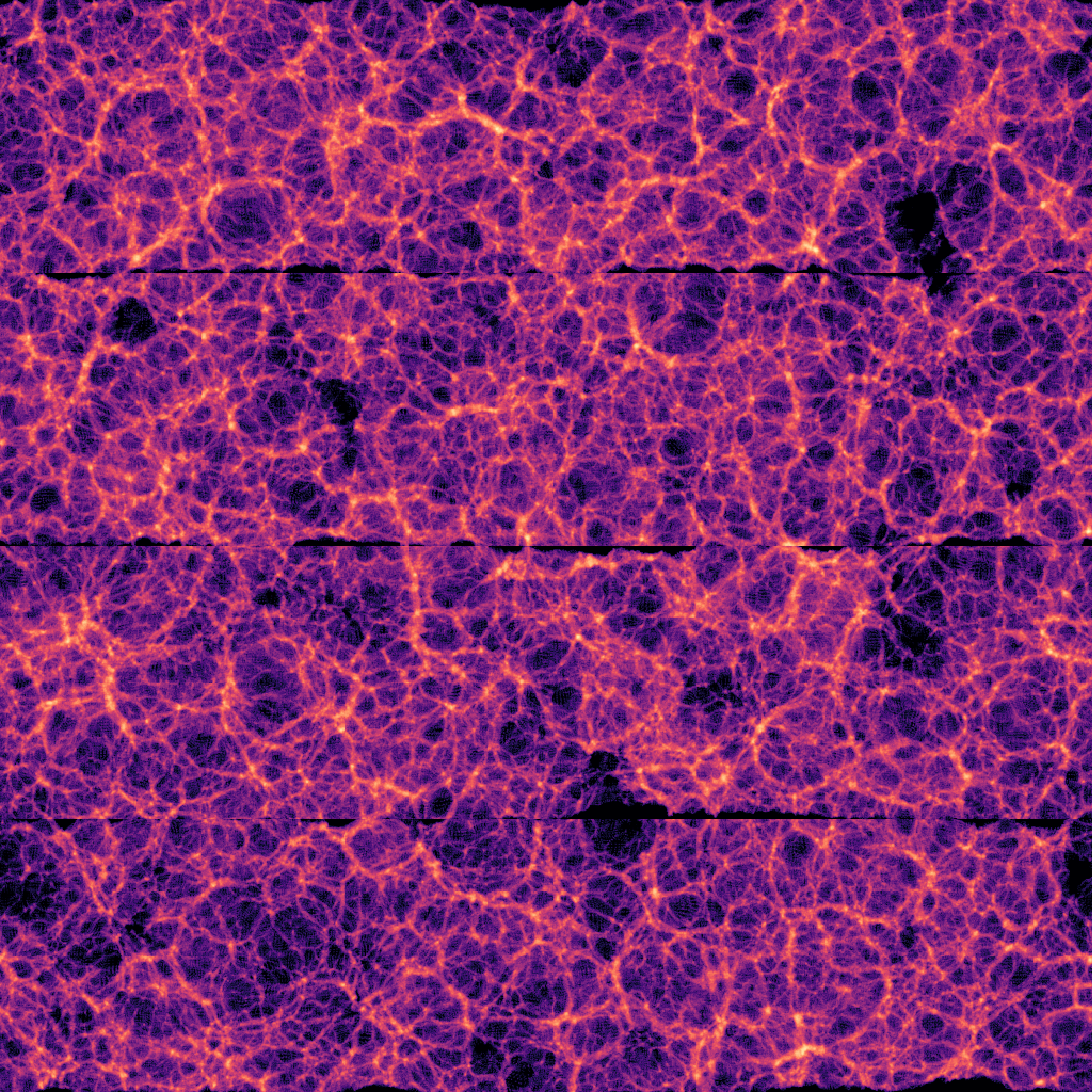
Without Halo Exchange (Not Distributed)

Sub Domain 1 (Particles)

Sub Domain 1 (Grid)

Sub Domain 1 (Read out)

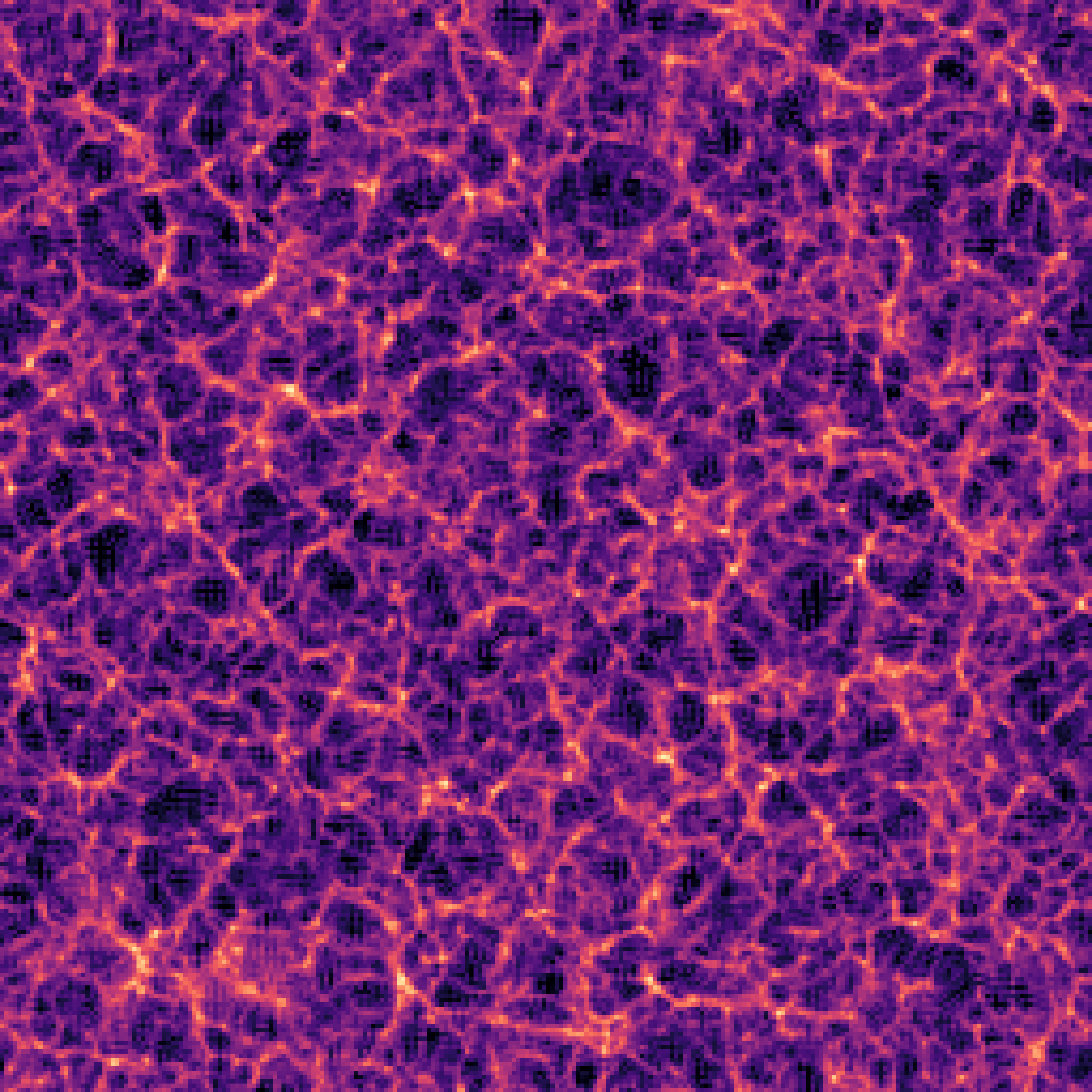
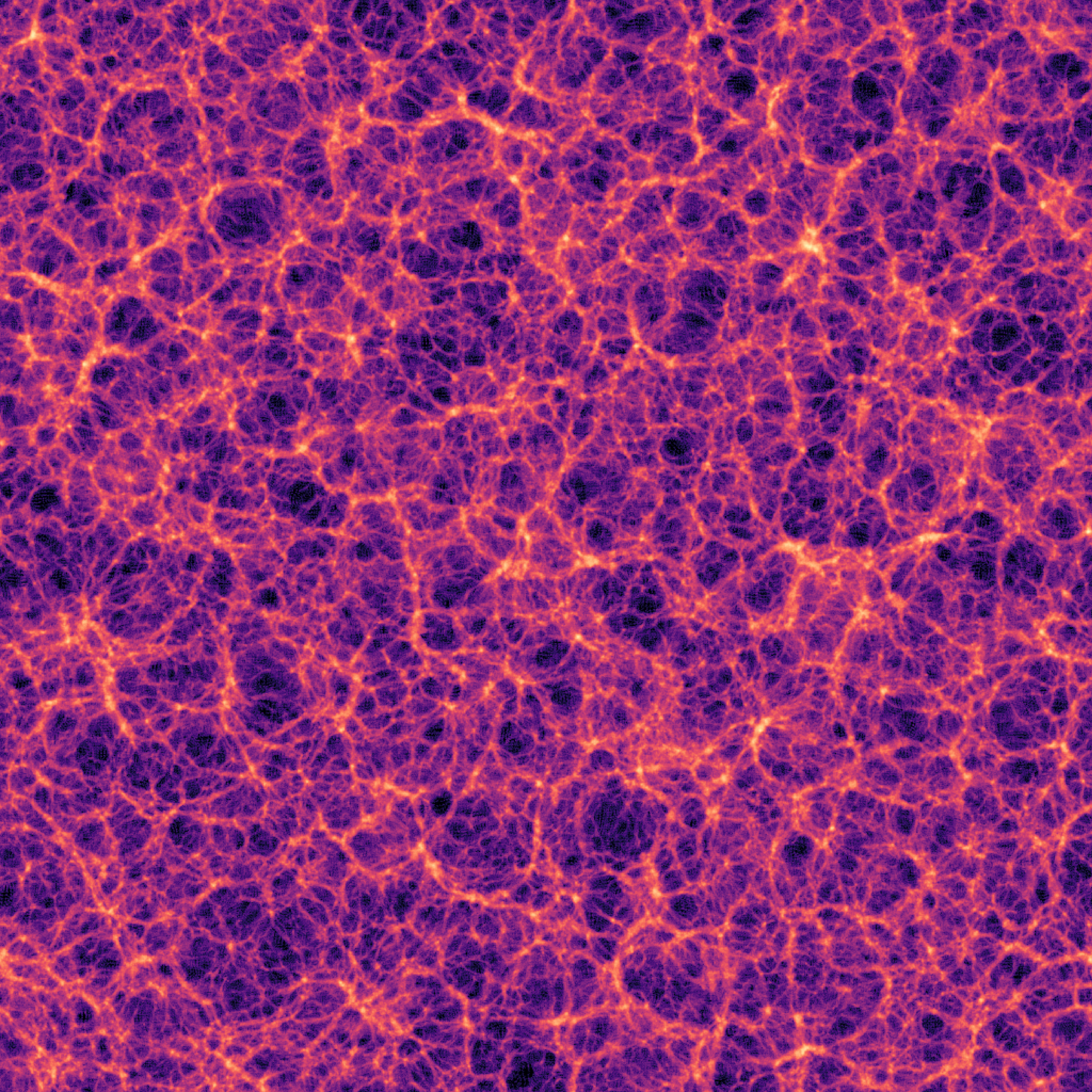
With Halo Exchange (Distributed)

Sub Domain 1 & Halo (Particles)

Sub Domain 1 & Halo (Grid)

Sub Domain 2 & Halo (Grid)

Why Halo Exchange Matters in Distributed Simulations

Without halo exchange, subdomain boundaries introduce visible artifacts in the final field.
This breaks the smoothness of the result — even when each local computation is correct.

First slice

Second slice

Third slice

Fourth slice

No Halo Artifacts

First slice

Second slice

Third slice

Fourth slice

With Halo no Artifacts

What About the Gradients?

Backpropagating Through ODE Integration

Why Gradients Are Costly

To compute gradients through a simulation, we need to track:

• All intermediate positions: \(d_i\)
• All velocities: \(v_i\)
• And their tangent vectors for backpropagation

Even though each update is simple, autodiff requires storing the full history.

Example: Kick-Drift Integration

A typical update step looks like:

\[ \begin{aligned} d_{i+1} &= d_i + v_i \, \Delta t \\\\ v_{i+1} &= v_i + F(d_{i+1}) \, \Delta t \end{aligned} \]

Over many steps, the memory demand scales linearly — which becomes a bottleneck for large simulations.

Why This Is a Problem in Practice

• Storing intermediate states for autodiff causes memory to scale linearly with the number of steps.

• Example costs at full resolution:

  • (1 Gpc/h)³, 10 steps → ~500 GB
  • (2 Gpc/h)³, 10 steps → ~4.2 TB

• This severely limits how many time steps or how large a volume we can afford — even with many GPUs.

Reverse Adjoint: Gradient Propagation Without Trajectory Storage (Preliminary)

• Instead of storing the full trajectory…

• We use the reverse adjoint method:

  • Save only the final state
  • Re-integrate backward in time to compute gradients

Forward Pass (Kick-Drift)

\[ \begin{aligned} d_{i+1} &= d_i + v_i \, \Delta t \\ v_{i+1} &= v_i + F(d_{i+1}) \, \Delta t \end{aligned} \]

Reverse Pass (Adjoint Method)

\[ \begin{aligned} v_i &= v_{i+1} - F(d_{i+1}) \, \Delta t \\ d_i &= d_{i+1} - v_i \, \Delta t \end{aligned} \]

Memory vs. Checkpoints

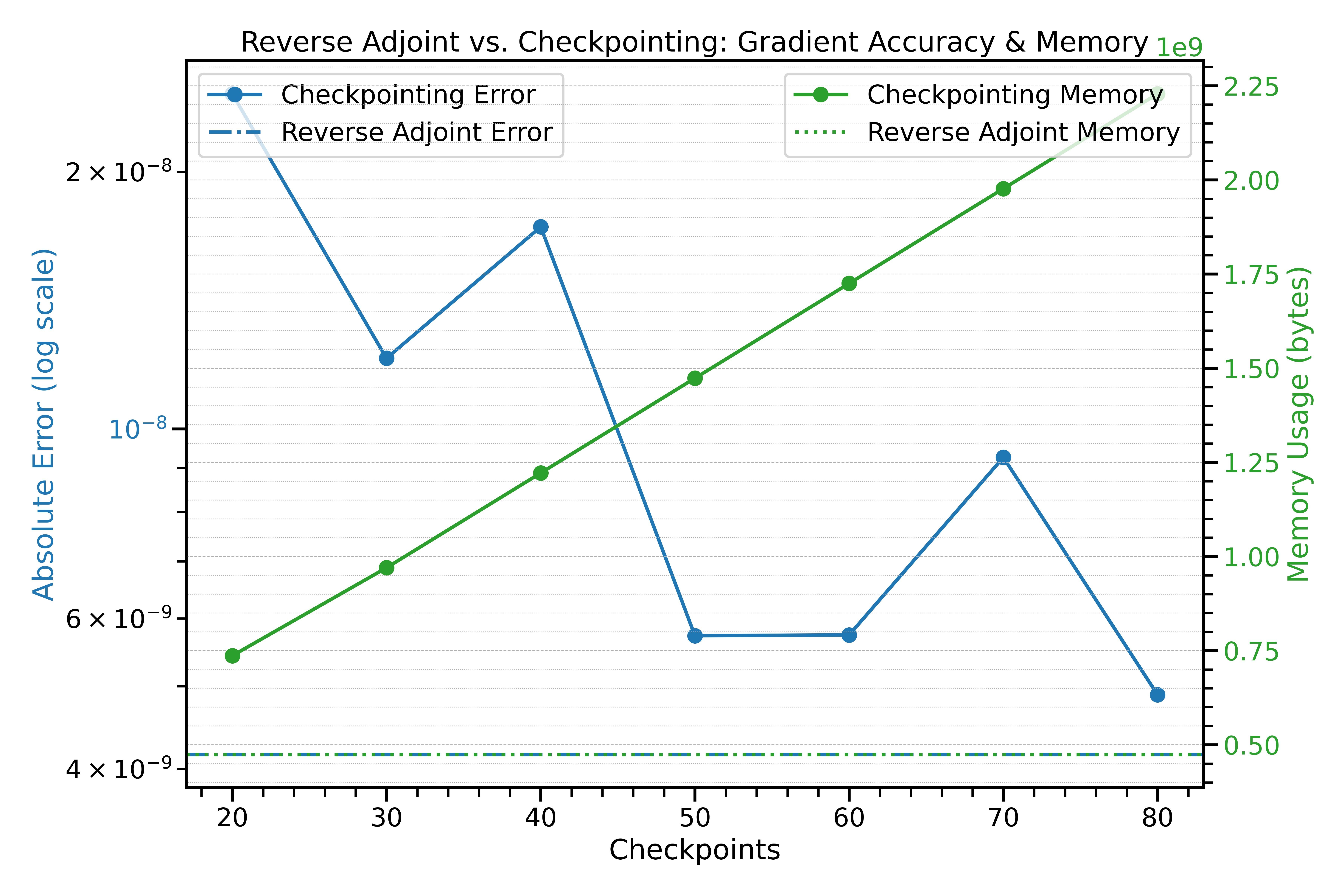
• Checkpointing saves intermediate simulation states periodically to reduce memory — but still grows with the number of steps.
• Reverse Adjoint recomputes on demand, keeping memory constant.

Reverse Adjoint Method

• Constant memory regardless of number of steps
• Requires a second simulation pass for gradient computation
• In a 10-step 1024³ Lightcone simulation, reverse adjoint uses 5× less memory than checkpointing (∼100 GB vs ∼500 GB)

Putting It All Together

JAXPM v0.1.5: Differentiable, Scalable Simulations

What JAXPM v0.1.5 Supports

• Multi-GPU and Multi-Node simulation with distributed domain decomposition (Successfully ran 2048³ on 256 GPUs)

• End-to-end differentiability, including force computation and interpolation

• Compatible with a custom JAX compatible Reverse Adjoint solver for memory-efficient gradients

• Supports full PM Lightcone Weak Lensing

• Available on PyPI: pip install jaxpm

• Built on top of jaxdecomp for distributed 3D FFT

Current Capabilities & Road Ahead

What We’ve Achieved So Far

• Built a scalable, differentiable N-body simulation pipeline (JAXPM)

• Enables forward modeling and sampling in large cosmological volumes, paving the way toward full LSST-scale inference

• Preliminary performance:

  • ~20 s per 512×512×1024 simulation on 64×A100 GPUs
  • <1 TB memory for full 10-step lightcone
  • Stable gradients over 100-sample tests

For discussion

• Using Scattering Transform to compress the data with SBI

• Using Excplicit Inference for CMB r estimation

Extra slides

Approximating the Small Scales

Dynamic resultion grid

•  We can use a dynamic resolution that automatically refines the grid to match the density regaions blabla
•   very difficult to differentialte and slow to compute

Dynamic Resolution Grid

Multigrid Methods

•  Multigrid solves the Poisson equation efficiently by combining coarse and fine grids
•  It’s still an approximation — it does not match the accuracy of solving on a uniformly fine grid
•  At high fidelity, fine-grid solvers outperform multigrid in recovering small-scale structure — critical for unbiased inference

Multigrid